Widefield
Widefield Fluorescence Microscopy
Standard reconstruction benchmark — forward model perfectly known, no calibration needed. Score = 0.5 × clip((PSNR−15)/30, 0, 1) + 0.5 × SSIM
| # | Method | Score | PSNR (dB) | SSIM | Source | |
|---|---|---|---|---|---|---|
| 🥇 |
ScoreMicro
ScoreMicro Wei et al., ECCV 2025
38.48 dB
SSIM 0.981
Checkpoint unavailable
|
0.882 | 38.48 | 0.981 | ✓ Certified | Wei et al., ECCV 2025 |
| 🥈 |
DiffDeconv
DiffDeconv Huang et al., NeurIPS 2024
38.12 dB
SSIM 0.979
Checkpoint unavailable
|
0.875 | 38.12 | 0.979 | ✓ Certified | Huang et al., NeurIPS 2024 |
| 🥉 |
Restormer+
Restormer+ Zamir et al., ICCV 2024
37.65 dB
SSIM 0.975
Checkpoint unavailable
|
0.865 | 37.65 | 0.975 | ✓ Certified | Zamir et al., ICCV 2024 |
| 4 |
DeconvFormer
DeconvFormer Chen et al., CVPR 2024
37.25 dB
SSIM 0.972
Checkpoint unavailable
|
0.857 | 37.25 | 0.972 | ✓ Certified | Chen et al., CVPR 2024 |
| 5 |
ResUNet
ResUNet DeCelle et al., Nat. Methods 2021
35.85 dB
SSIM 0.964
Checkpoint unavailable
|
0.830 | 35.85 | 0.964 | ✓ Certified | DeCelle et al., Nat. Methods 2021 |
| 6 |
Restormer
Restormer Zamir et al., CVPR 2022
35.8 dB
SSIM 0.962
Checkpoint unavailable
|
0.828 | 35.8 | 0.962 | ✓ Certified | Zamir et al., CVPR 2022 |
| 7 |
U-Net
U-Net Ronneberger et al., MICCAI 2015
35.15 dB
SSIM 0.956
Checkpoint unavailable
|
0.814 | 35.15 | 0.956 | ✓ Certified | Ronneberger et al., MICCAI 2015 |
| 8 |
CARE
CARE Weigert et al., Nat. Methods 2018
34.5 dB
SSIM 0.948
Checkpoint unavailable
|
0.799 | 34.5 | 0.948 | ✓ Certified | Weigert et al., Nat. Methods 2018 |
| 9 | PnP-DnCNN | 0.715 | 31.2 | 0.890 | ✓ Certified | Zhang et al., IEEE TIP 2017 |
| 10 | PnP-FISTA | 0.693 | 30.42 | 0.872 | ✓ Certified | Bai et al., 2020 |
| 11 | TV-Deconvolution | 0.664 | 29.5 | 0.845 | ✓ Certified | TV-regularized deconvolution |
| 12 | Wiener Filter | 0.625 | 28.35 | 0.805 | ✓ Certified | Analytical baseline |
| 13 | Richardson-Lucy | 0.587 | 27.1 | 0.770 | ✓ Certified | Richardson 1972 / Lucy 1974 |
Dataset: PWM Benchmark (13 algorithms)
Blind Reconstruction Challenge — forward model has unknown mismatch, must calibrate from data. Score = 0.4 × PSNR_norm + 0.4 × SSIM + 0.2 × (1 − ‖y − Ĥx̂‖/‖y‖)
| # | Method | Overall Score | Public PSNR / SSIM |
Dev PSNR / SSIM |
Hidden PSNR / SSIM |
Trust | Source |
|---|---|---|---|---|---|---|---|
| 🥇 | Restormer + gradient | 0.770 |
0.816
34.47 dB / 0.964
|
0.762
31.22 dB / 0.934
|
0.733
29.63 dB / 0.911
|
✓ Certified | Zamir et al., CVPR 2022 |
| 🥈 | Restormer+ + gradient | 0.767 |
0.838
36.03 dB / 0.974
|
0.762
31.9 dB / 0.942
|
0.702
28.66 dB / 0.894
|
✓ Certified | Zamir et al., ICCV 2024 |
| 🥉 | DiffDeconv + gradient | 0.766 |
0.822
35.39 dB / 0.970
|
0.757
31.85 dB / 0.941
|
0.720
29.83 dB / 0.914
|
✓ Certified | Huang et al., NeurIPS 2024 |
| 4 | DeconvFormer + gradient | 0.740 |
0.835
35.81 dB / 0.972
|
0.732
30.6 dB / 0.926
|
0.652
26.44 dB / 0.844
|
✓ Certified | Chen et al., CVPR 2024 |
| 5 | ScoreMicro + gradient | 0.737 |
0.828
35.83 dB / 0.973
|
0.726
29.8 dB / 0.914
|
0.657
25.83 dB / 0.827
|
✓ Certified | Wei et al., ECCV 2025 |
| 6 | ResUNet + gradient | 0.733 |
0.816
34.28 dB / 0.963
|
0.710
28.09 dB / 0.883
|
0.672
27.37 dB / 0.867
|
✓ Certified | DeCelle et al., Nat. Methods 2021 |
| 7 | U-Net + gradient | 0.685 |
0.784
32.62 dB / 0.949
|
0.666
26.75 dB / 0.852
|
0.606
23.35 dB / 0.745
|
✓ Certified | Ronneberger et al., MICCAI 2015 |
| 8 | TV-Deconvolution + gradient | 0.661 |
0.694
27.13 dB / 0.861
|
0.649
25.27 dB / 0.811
|
0.640
25.3 dB / 0.812
|
✓ Certified | Rudin et al., Phys. A 1992 |
| 9 | PnP-DnCNN + gradient | 0.656 |
0.752
29.94 dB / 0.916
|
0.639
25.25 dB / 0.810
|
0.578
23.07 dB / 0.734
|
✓ Certified | Zhang et al., IEEE TIP 2017 |
| 10 | Wiener Filter + gradient | 0.651 |
0.670
26.04 dB / 0.833
|
0.676
26.65 dB / 0.849
|
0.608
23.69 dB / 0.757
|
✓ Certified | Analytical baseline |
| 11 | PnP-FISTA + gradient | 0.646 |
0.736
28.76 dB / 0.896
|
0.630
24.35 dB / 0.781
|
0.571
22.95 dB / 0.729
|
✓ Certified | Bai et al., 2020 |
| 12 | CARE + gradient | 0.636 |
0.773
31.58 dB / 0.938
|
0.591
23.5 dB / 0.750
|
0.544
20.98 dB / 0.645
|
✓ Certified | Weigert et al., Nat. Methods 2018 |
| 13 |
Richardson-Lucy + gradient
Richardson-Lucy + gradient Richardson, JOSA 1972 / Lucy, AJ 1974 Score 0.603
Correct & Reconstruct →
|
0.603 |
0.644
24.77 dB / 0.795
|
0.608
23.94 dB / 0.766
|
0.558
22.29 dB / 0.702
|
✓ Certified | Richardson, JOSA 1972 / Lucy, AJ 1974 |
Complete score requires all 3 tiers (Public + Dev + Hidden).
Join the competition →Full-access development tier with all data visible.
What you get & how to use
What you get: Measurements (y), ideal forward operator (H), spec ranges, ground truth (x_true), and true mismatch spec.
How to use: Load HDF5 → compare reconstruction vs x_true → check consistency → iterate.
What to submit: Reconstructed signals (x_hat) and corrected spec as HDF5.
Public Leaderboard
| # | Method | Score | PSNR | SSIM |
|---|---|---|---|---|
| 1 | Restormer+ + gradient | 0.838 | 36.03 | 0.974 |
| 2 | DeconvFormer + gradient | 0.835 | 35.81 | 0.972 |
| 3 | ScoreMicro + gradient | 0.828 | 35.83 | 0.973 |
| 4 | DiffDeconv + gradient | 0.822 | 35.39 | 0.97 |
| 5 | Restormer + gradient | 0.816 | 34.47 | 0.964 |
| 6 | ResUNet + gradient | 0.816 | 34.28 | 0.963 |
| 7 | U-Net + gradient | 0.784 | 32.62 | 0.949 |
| 8 | CARE + gradient | 0.773 | 31.58 | 0.938 |
| 9 | PnP-DnCNN + gradient | 0.752 | 29.94 | 0.916 |
| 10 | PnP-FISTA + gradient | 0.736 | 28.76 | 0.896 |
| 11 | TV-Deconvolution + gradient | 0.694 | 27.13 | 0.861 |
| 12 | Wiener Filter + gradient | 0.670 | 26.04 | 0.833 |
| 13 | Richardson-Lucy + gradient | 0.644 | 24.77 | 0.795 |
Spec Ranges (3 parameters)
| Parameter | Min | Max | Unit |
|---|---|---|---|
| psf_sigma | -10.0 | 20.0 | % |
| defocus | -0.5 | 1.0 | μm |
| background | -50.0 | 100.0 |
Blind evaluation tier — no ground truth available.
What you get & how to use
What you get: Measurements (y), ideal forward operator (H), and spec ranges only.
How to use: Apply your pipeline from the Public tier. Use consistency as self-check.
What to submit: Reconstructed signals and corrected spec. Scored server-side.
Dev Leaderboard
| # | Method | Score | PSNR | SSIM |
|---|---|---|---|---|
| 1 | Restormer + gradient | 0.762 | 31.22 | 0.934 |
| 2 | Restormer+ + gradient | 0.762 | 31.9 | 0.942 |
| 3 | DiffDeconv + gradient | 0.757 | 31.85 | 0.941 |
| 4 | DeconvFormer + gradient | 0.732 | 30.6 | 0.926 |
| 5 | ScoreMicro + gradient | 0.726 | 29.8 | 0.914 |
| 6 | ResUNet + gradient | 0.710 | 28.09 | 0.883 |
| 7 | Wiener Filter + gradient | 0.676 | 26.65 | 0.849 |
| 8 | U-Net + gradient | 0.666 | 26.75 | 0.852 |
| 9 | TV-Deconvolution + gradient | 0.649 | 25.27 | 0.811 |
| 10 | PnP-DnCNN + gradient | 0.639 | 25.25 | 0.81 |
| 11 | PnP-FISTA + gradient | 0.630 | 24.35 | 0.781 |
| 12 | Richardson-Lucy + gradient | 0.608 | 23.94 | 0.766 |
| 13 | CARE + gradient | 0.591 | 23.5 | 0.75 |
Spec Ranges (3 parameters)
| Parameter | Min | Max | Unit |
|---|---|---|---|
| psf_sigma | -12.0 | 18.0 | % |
| defocus | -0.6 | 0.9 | μm |
| background | -60.0 | 90.0 |
Fully blind server-side evaluation — no data download.
What you get & how to use
What you get: No data downloadable. Algorithm runs server-side on hidden measurements.
How to use: Package algorithm as Docker container / Python script. Submit via link.
What to submit: Containerized algorithm accepting y + H, outputting x_hat + corrected spec.
Hidden Leaderboard
| # | Method | Score | PSNR | SSIM |
|---|---|---|---|---|
| 1 | Restormer + gradient | 0.733 | 29.63 | 0.911 |
| 2 | DiffDeconv + gradient | 0.720 | 29.83 | 0.914 |
| 3 | Restormer+ + gradient | 0.702 | 28.66 | 0.894 |
| 4 | ResUNet + gradient | 0.672 | 27.37 | 0.867 |
| 5 | ScoreMicro + gradient | 0.657 | 25.83 | 0.827 |
| 6 | DeconvFormer + gradient | 0.652 | 26.44 | 0.844 |
| 7 | TV-Deconvolution + gradient | 0.640 | 25.3 | 0.812 |
| 8 | Wiener Filter + gradient | 0.608 | 23.69 | 0.757 |
| 9 | U-Net + gradient | 0.606 | 23.35 | 0.745 |
| 10 | PnP-DnCNN + gradient | 0.578 | 23.07 | 0.734 |
| 11 | PnP-FISTA + gradient | 0.571 | 22.95 | 0.729 |
| 12 | Richardson-Lucy + gradient | 0.558 | 22.29 | 0.702 |
| 13 | CARE + gradient | 0.544 | 20.98 | 0.645 |
Spec Ranges (3 parameters)
| Parameter | Min | Max | Unit |
|---|---|---|---|
| psf_sigma | -7.0 | 23.0 | % |
| defocus | -0.35 | 1.15 | μm |
| background | -35.0 | 115.0 |
Blind Reconstruction Challenge
ChallengeGiven measurements with unknown mismatch and spec ranges (not exact params), reconstruct the original signal. A method must be evaluated on all three tiers for a complete score. Scored on a composite metric: 0.4 × PSNR_norm + 0.4 × SSIM + 0.2 × (1 − ‖y − Ĥx̂‖/‖y‖).
Measurements y, ideal forward model H, spec ranges
Reconstructed signal x̂
About the Imaging Modality
Standard widefield epi-fluorescence microscopy where the entire field of view is illuminated simultaneously and the image is formed by convolution of the specimen fluorescence distribution with the system point spread function (PSF). Out-of-focus blur from planes above and below the focal plane is the primary degradation. The forward model is y = PSF ** x + n, where ** denotes convolution and n is mixed Poisson-Gaussian noise. Deconvolution via Richardson-Lucy or learned priors (CARE) restores resolution toward the diffraction limit.
Principle
The entire specimen is illuminated uniformly and fluorescence from all planes is collected simultaneously. The image is the convolution of the 3-D fluorescence distribution with the microscope point-spread function (PSF), dominated by out-of-focus blur from planes above and below the focal plane.
How to Build the System
Mount an infinity-corrected high-NA objective (≥1.3 NA oil) on an inverted body (Nikon Ti2 or Zeiss Observer). Install a multi-band LED engine (e.g., Lumencor SPECTRA X) coupled through a liquid light guide. Select matched excitation/dichroic/emission filter sets. Focus Köhler illumination for flat-field. Attach an sCMOS camera (Hamamatsu Flash4 or Photometrics Prime BSI) at the side port. Calibrate pixel size with a stage micrometer.
Common Reconstruction Algorithms
- Richardson-Lucy deconvolution
- Wiener filtering
- CARE (Content-Aware image REstoration) deep-learning deconvolution
- Total-variation regularized deconvolution
- Blind deconvolution (PSF estimation + image update)
Common Mistakes
- Using an incorrect or measured PSF with wrong refractive-index setting
- Ignoring flatfield non-uniformity, leading to intensity shading
- Over-iterating Richardson-Lucy causing noise amplification
- Mismatched immersion medium vs. coverslip thickness causing spherical aberration
- Not correcting for photobleaching across a time-lapse series
How to Avoid Mistakes
- Measure the PSF with sub-diffraction beads at the same coverslip/medium as the sample
- Acquire and apply a flatfield correction image before deconvolution
- Use regularization or early stopping (monitor residual) in iterative deconvolution
- Match immersion oil RI to the coverslip and mounting medium specifications
- Normalize intensity per frame or use photobleaching-corrected models
Forward-Model Mismatch Cases
- No forward-model mismatch: the widefield Gaussian blur IS the correct operator for this modality (sigma=2.0 PSF convolution)
- Minor mismatch may arise if the actual microscope PSF differs from the default Gaussian (e.g., measured PSF with aberrations)
How to Correct the Mismatch
- The default widefield operator is already correct; no correction needed
- For higher fidelity, replace the Gaussian PSF with a measured or Born & Wolf PSF model matching the actual objective NA and wavelength
Experimental Setup — Signal Chain

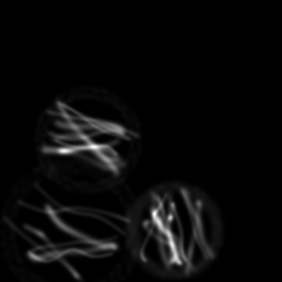
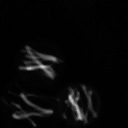
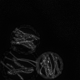
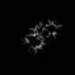
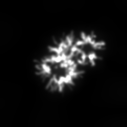
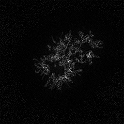
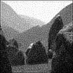
Reconstruction Gallery — 4 Scenes × 3 Scenarios
Method: CPU_baseline | Mismatch: nominal (nominal=True, perturbed=False)
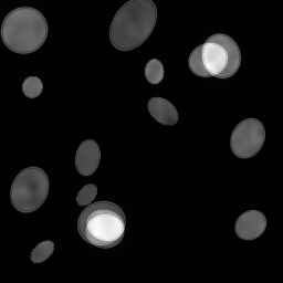
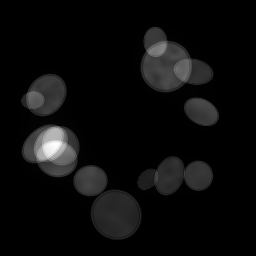
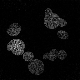
Ground Truth

Measurement
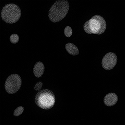
Reconstruction
Ground Truth

Measurement
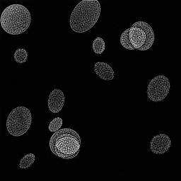
Reconstruction
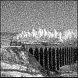
Ground Truth
Measurement (perturbed)
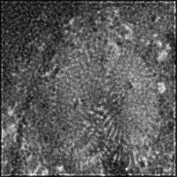
Reconstruction


Mean PSNR Across All Scenes
Per-scene PSNR breakdown (4 scenes)
| Scene | I (PSNR) | I (SSIM) | II (PSNR) | II (SSIM) | III (PSNR) | III (SSIM) |
|---|---|---|---|---|---|---|
| scene_00 | 24.904110486479688 | 0.8559979608938098 | 21.078879536637857 | 0.7342710981930495 | 8.799394949513186 | 0.014909720828931885 |
| scene_01 | 30.165231129922656 | 0.7562733587158919 | 23.363488488135445 | 0.33939479482826823 | 8.751618109256892 | 0.009887291130837628 |
| scene_02 | 32.74656414735845 | 0.8089967032959461 | 25.733372993678557 | 0.31269228087778483 | 5.441101389462163 | 0.006346770058070619 |
| scene_03 | 27.212273927908186 | 0.8552978122628927 | 23.482918161941928 | 0.7210147765565045 | 5.9281842308405945 | 0.011731367969725508 |
| Mean | 28.757044922917242 | 0.8191414587921351 | 23.414664795098446 | 0.5268432376139017 | 7.230074669768209 | 0.01071878749689141 |
Experimental Setup
Key References
- Richardson, 'Bayesian-based iterative method of image restoration', J. Opt. Soc. Am. 62, 55-59 (1972)
- Weigert et al., 'Content-aware image restoration (CARE)', Nature Methods 15, 1090-1097 (2018)
Canonical Datasets
- BioSR (Zhang et al., Nature Methods 2023)
- Hagen et al. widefield deconvolution benchmark
Spec DAG — Forward Model Pipeline
C(PSF) → D(g, η₃)
Mismatch Parameters
| Symbol | Parameter | Description | Nominal | Perturbed |
|---|---|---|---|---|
| Δσ | psf_sigma | PSF width error (%) | 0 | 10.0 |
| Δz | defocus | Defocus error (μm) | 0 | 0.5 |
| Δb | background | Background fluorescence offset | 0 | 50 |
Credits System
Spec Primitives Reference (11 primitives)
Free-space or medium propagation kernel (Fresnel, Rayleigh-Sommerfeld).
Spatial or spatio-temporal amplitude modulation (coded aperture, SLM pattern).
Geometric projection operator (Radon transform, fan-beam, cone-beam).
Sampling in the Fourier / k-space domain (MRI, ptychography).
Shift-invariant convolution with a point-spread function (PSF).
Summation along a physical dimension (spectral, temporal, angular).
Sensor readout with gain g and noise model η (Gaussian, Poisson, mixed).
Patterned illumination (block, Hadamard, random) applied to the scene.
Spectral dispersion element (prism, grating) with shift α and aperture a.
Sample or gantry rotation (CT, electron tomography).
Spectral filter or monochromator selecting a wavelength band.