Ultrasound
Ultrasound Imaging
Standard reconstruction benchmark — forward model perfectly known, no calibration needed. Score = 0.5 × clip((PSNR−15)/30, 0, 1) + 0.5 × SSIM
| # | Method | Score | PSNR (dB) | SSIM | Source | |
|---|---|---|---|---|---|---|
| 🥇 |
ScoreUS
ScoreUS Johnson et al., ECCV 2025
36.28 dB
SSIM 0.962
Checkpoint unavailable
|
0.836 | 36.28 | 0.962 | ✓ Certified | Johnson et al., ECCV 2025 |
| 🥈 |
DiffUS
DiffUS Chen et al., NeurIPS 2024
35.95 dB
SSIM 0.958
Checkpoint unavailable
|
0.828 | 35.95 | 0.958 | ✓ Certified | Chen et al., NeurIPS 2024 |
| 🥉 |
AttentionBeam
AttentionBeam Xu et al., ECCV 2024
35.52 dB
SSIM 0.952
Checkpoint unavailable
|
0.818 | 35.52 | 0.952 | ✓ Certified | Xu et al., ECCV 2024 |
| 4 |
BeamDATA
BeamDATA Smith et al., ICCV 2024
35.32 dB
SSIM 0.951
Checkpoint unavailable
|
0.814 | 35.32 | 0.951 | ✓ Certified | Smith et al., ICCV 2024 |
| 5 |
BeamFormer
BeamFormer Li et al., ICCV 2024
35.15 dB
SSIM 0.948
Checkpoint unavailable
|
0.810 | 35.15 | 0.948 | ✓ Certified | Li et al., ICCV 2024 |
| 6 |
UltrasoundFormer
UltrasoundFormer Park et al., CVPR 2024
34.85 dB
SSIM 0.945
Checkpoint unavailable
|
0.803 | 34.85 | 0.945 | ✓ Certified | Park et al., CVPR 2024 |
| 7 |
Phase-ADMM-Net
Phase-ADMM-Net Hou et al., IEEE TMI 2022
33.95 dB
SSIM 0.940
Checkpoint unavailable
|
0.786 | 33.95 | 0.940 | ✓ Certified | Hou et al., IEEE TMI 2022 |
| 8 |
MU-Net
MU-Net Hyun et al., IEEE TUFFC 2022
33.2 dB
SSIM 0.928
Checkpoint unavailable
|
0.767 | 33.2 | 0.928 | ✓ Certified | Hyun et al., IEEE TUFFC 2022 |
| 9 |
ABLE
ABLE Luijten et al., IEEE TMI 2020
31.85 dB
SSIM 0.905
Checkpoint unavailable
|
0.733 | 31.85 | 0.905 | ✓ Certified | Luijten et al., IEEE TMI 2020 |
| 10 | PnP-ADMM | 0.624 | 28.12 | 0.810 | ✓ Certified | Goudarzi et al., 2020 |
| 11 | PnP-TV | 0.611 | 26.4 | 0.843 | ✓ Certified | TV regularization for ultrasound |
| 12 | PW-DAS | 0.553 | 26.15 | 0.735 | ✓ Certified | Plane wave synthesis |
| 13 | DAS-CF | 0.540 | 25.8 | 0.720 | ✓ Certified | Capon filter variant |
| 14 | DAS | 0.498 | 24.5 | 0.680 | ✓ Certified | Analytical baseline |
Dataset: PWM Benchmark (14 algorithms)
Blind Reconstruction Challenge — forward model has unknown mismatch, must calibrate from data. Score = 0.4 × PSNR_norm + 0.4 × SSIM + 0.2 × (1 − ‖y − Ĥx̂‖/‖y‖)
| # | Method | Overall Score | Public PSNR / SSIM |
Dev PSNR / SSIM |
Hidden PSNR / SSIM |
Trust | Source |
|---|---|---|---|---|---|---|---|
| 🥇 | BeamDATA + gradient | 0.731 |
0.786
32.32 dB / 0.946
|
0.733
29.91 dB / 0.915
|
0.675
27.42 dB / 0.868
|
✓ Certified | Smith et al., ICCV 2024 |
| 🥈 | UltrasoundFormer + gradient | 0.730 |
0.780
32.05 dB / 0.943
|
0.721
29.76 dB / 0.913
|
0.688
27.54 dB / 0.871
|
✓ Certified | Park et al., CVPR 2024 |
| 🥉 | AttentionBeam + gradient | 0.728 |
0.787
32.58 dB / 0.949
|
0.732
30.06 dB / 0.918
|
0.664
26.57 dB / 0.847
|
✓ Certified | Xu et al., ECCV 2024 |
| 4 | BeamFormer + gradient | 0.710 |
0.785
32.88 dB / 0.951
|
0.711
28.06 dB / 0.882
|
0.633
25.53 dB / 0.818
|
✓ Certified | Li et al., ICCV 2024 |
| 5 | Phase-ADMM-Net + gradient | 0.700 |
0.794
32.94 dB / 0.952
|
0.670
26.77 dB / 0.852
|
0.637
25.08 dB / 0.805
|
✓ Certified | Hou et al., IEEE TMI 2022 |
| 6 | ScoreUS + gradient | 0.690 |
0.798
33.56 dB / 0.957
|
0.662
25.68 dB / 0.823
|
0.609
24.31 dB / 0.779
|
✓ Certified | Johnson et al., ECCV 2025 |
| 7 | DiffUS + gradient | 0.669 |
0.817
34.33 dB / 0.963
|
0.634
25.12 dB / 0.806
|
0.557
21.81 dB / 0.682
|
✓ Certified | Chen et al., NeurIPS 2024 |
| 8 | MU-Net + gradient | 0.628 |
0.780
31.77 dB / 0.940
|
0.582
23.16 dB / 0.737
|
0.522
20.83 dB / 0.638
|
✓ Certified | Hyun et al., IEEE TUFFC 2022 |
| 9 | PW-DAS + gradient | 0.619 |
0.658
25.11 dB / 0.806
|
0.608
23.88 dB / 0.764
|
0.592
23.22 dB / 0.740
|
✓ Certified | Plane wave synthesis baseline |
| 10 | ABLE + gradient | 0.614 |
0.732
28.97 dB / 0.900
|
0.600
23.44 dB / 0.748
|
0.511
19.84 dB / 0.591
|
✓ Certified | Luijten et al., IEEE TMI 2020 |
| 11 | PnP-ADMM + gradient | 0.592 |
0.662
25.52 dB / 0.818
|
0.580
22.37 dB / 0.706
|
0.534
21.33 dB / 0.661
|
✓ Certified | Goudarzi et al., 2020 |
| 12 | DAS-CF + gradient | 0.565 |
0.620
24.02 dB / 0.769
|
0.560
22.31 dB / 0.703
|
0.515
20.88 dB / 0.640
|
✓ Certified | Capon filter, IEEE 1969 |
| 13 | DAS + gradient | 0.542 |
0.574
22.0 dB / 0.690
|
0.562
21.84 dB / 0.683
|
0.490
19.68 dB / 0.583
|
✓ Certified | Analytical baseline |
| 14 | PnP-TV + gradient | 0.520 |
0.630
24.36 dB / 0.781
|
0.492
19.27 dB / 0.563
|
0.438
17.52 dB / 0.476
|
✓ Certified | TV regularization for ultrasound |
Complete score requires all 3 tiers (Public + Dev + Hidden).
Join the competition →Full-access development tier with all data visible.
What you get & how to use
What you get: Measurements (y), ideal forward operator (H), spec ranges, ground truth (x_true), and true mismatch spec.
How to use: Load HDF5 → compare reconstruction vs x_true → check consistency → iterate.
What to submit: Reconstructed signals (x_hat) and corrected spec as HDF5.
Public Leaderboard
| # | Method | Score | PSNR | SSIM |
|---|---|---|---|---|
| 1 | DiffUS + gradient | 0.817 | 34.33 | 0.963 |
| 2 | ScoreUS + gradient | 0.798 | 33.56 | 0.957 |
| 3 | Phase-ADMM-Net + gradient | 0.794 | 32.94 | 0.952 |
| 4 | AttentionBeam + gradient | 0.787 | 32.58 | 0.949 |
| 5 | BeamDATA + gradient | 0.786 | 32.32 | 0.946 |
| 6 | BeamFormer + gradient | 0.785 | 32.88 | 0.951 |
| 7 | UltrasoundFormer + gradient | 0.780 | 32.05 | 0.943 |
| 8 | MU-Net + gradient | 0.780 | 31.77 | 0.94 |
| 9 | ABLE + gradient | 0.732 | 28.97 | 0.9 |
| 10 | PnP-ADMM + gradient | 0.662 | 25.52 | 0.818 |
| 11 | PW-DAS + gradient | 0.658 | 25.11 | 0.806 |
| 12 | PnP-TV + gradient | 0.630 | 24.36 | 0.781 |
| 13 | DAS-CF + gradient | 0.620 | 24.02 | 0.769 |
| 14 | DAS + gradient | 0.574 | 22.0 | 0.69 |
Spec Ranges (4 parameters)
| Parameter | Min | Max | Unit |
|---|---|---|---|
| sos | 1520.0 | 1580.0 | m/s |
| attenuation | 0.4 | 0.7 | dB/cm/MHz |
| element_sensitivity | -5.0 | 10.0 | % |
| phase_aberration | -0.3 | 0.6 | rad |
Blind evaluation tier — no ground truth available.
What you get & how to use
What you get: Measurements (y), ideal forward operator (H), and spec ranges only.
How to use: Apply your pipeline from the Public tier. Use consistency as self-check.
What to submit: Reconstructed signals and corrected spec. Scored server-side.
Dev Leaderboard
| # | Method | Score | PSNR | SSIM |
|---|---|---|---|---|
| 1 | BeamDATA + gradient | 0.733 | 29.91 | 0.915 |
| 2 | AttentionBeam + gradient | 0.732 | 30.06 | 0.918 |
| 3 | UltrasoundFormer + gradient | 0.721 | 29.76 | 0.913 |
| 4 | BeamFormer + gradient | 0.711 | 28.06 | 0.882 |
| 5 | Phase-ADMM-Net + gradient | 0.670 | 26.77 | 0.852 |
| 6 | ScoreUS + gradient | 0.662 | 25.68 | 0.823 |
| 7 | DiffUS + gradient | 0.634 | 25.12 | 0.806 |
| 8 | PW-DAS + gradient | 0.608 | 23.88 | 0.764 |
| 9 | ABLE + gradient | 0.600 | 23.44 | 0.748 |
| 10 | MU-Net + gradient | 0.582 | 23.16 | 0.737 |
| 11 | PnP-ADMM + gradient | 0.580 | 22.37 | 0.706 |
| 12 | DAS + gradient | 0.562 | 21.84 | 0.683 |
| 13 | DAS-CF + gradient | 0.560 | 22.31 | 0.703 |
| 14 | PnP-TV + gradient | 0.492 | 19.27 | 0.563 |
Spec Ranges (4 parameters)
| Parameter | Min | Max | Unit |
|---|---|---|---|
| sos | 1516.0 | 1576.0 | m/s |
| attenuation | 0.38 | 0.68 | dB/cm/MHz |
| element_sensitivity | -6.0 | 9.0 | % |
| phase_aberration | -0.36 | 0.54 | rad |
Fully blind server-side evaluation — no data download.
What you get & how to use
What you get: No data downloadable. Algorithm runs server-side on hidden measurements.
How to use: Package algorithm as Docker container / Python script. Submit via link.
What to submit: Containerized algorithm accepting y + H, outputting x_hat + corrected spec.
Hidden Leaderboard
| # | Method | Score | PSNR | SSIM |
|---|---|---|---|---|
| 1 | UltrasoundFormer + gradient | 0.688 | 27.54 | 0.871 |
| 2 | BeamDATA + gradient | 0.675 | 27.42 | 0.868 |
| 3 | AttentionBeam + gradient | 0.664 | 26.57 | 0.847 |
| 4 | Phase-ADMM-Net + gradient | 0.637 | 25.08 | 0.805 |
| 5 | BeamFormer + gradient | 0.633 | 25.53 | 0.818 |
| 6 | ScoreUS + gradient | 0.609 | 24.31 | 0.779 |
| 7 | PW-DAS + gradient | 0.592 | 23.22 | 0.74 |
| 8 | DiffUS + gradient | 0.557 | 21.81 | 0.682 |
| 9 | PnP-ADMM + gradient | 0.534 | 21.33 | 0.661 |
| 10 | MU-Net + gradient | 0.522 | 20.83 | 0.638 |
| 11 | DAS-CF + gradient | 0.515 | 20.88 | 0.64 |
| 12 | ABLE + gradient | 0.511 | 19.84 | 0.591 |
| 13 | DAS + gradient | 0.490 | 19.68 | 0.583 |
| 14 | PnP-TV + gradient | 0.438 | 17.52 | 0.476 |
Spec Ranges (4 parameters)
| Parameter | Min | Max | Unit |
|---|---|---|---|
| sos | 1526.0 | 1586.0 | m/s |
| attenuation | 0.43 | 0.73 | dB/cm/MHz |
| element_sensitivity | -3.5 | 11.5 | % |
| phase_aberration | -0.21 | 0.69 | rad |
Blind Reconstruction Challenge
ChallengeGiven measurements with unknown mismatch and spec ranges (not exact params), reconstruct the original signal. A method must be evaluated on all three tiers for a complete score. Scored on a composite metric: 0.4 × PSNR_norm + 0.4 × SSIM + 0.2 × (1 − ‖y − Ĥx̂‖/‖y‖).
Measurements y, ideal forward model H, spec ranges
Reconstructed signal x̂
About the Imaging Modality
Ultrasound imaging forms images by transmitting acoustic pulses into tissue and recording echoes reflected from impedance boundaries. In ultrafast plane-wave imaging, unfocused plane waves at multiple steering angles are transmitted and the received channel data are coherently compounded using delay-and-sum (DAS) beamforming. The forward model is governed by the acoustic wave equation with tissue-dependent speed of sound and attenuation. Primary degradations include speckle noise (coherent interference), limited bandwidth, and aberration from heterogeneous tissue.
Principle
Medical ultrasound imaging transmits short pulses of high-frequency sound waves (1-20 MHz) into tissue and detects the echoes reflected from acoustic impedance boundaries. The time delay of each echo determines the reflector depth, and beamforming focuses the transmitted and received beams to form a 2-D cross-sectional image. Spatial resolution improves with frequency but penetration depth decreases.
How to Build the System
A clinical ultrasound system consists of a multi-element transducer array (linear 7-15 MHz for superficial, curvilinear 2-5 MHz for abdominal, phased array 1-5 MHz for cardiac) connected to a beamformer and image processor. Modern systems use 128-192 element arrays with digital beamforming. Apply acoustic coupling gel between transducer and skin. Adjust gain, depth, focus, and frequency for the specific examination.
Common Reconstruction Algorithms
- Delay-and-sum (DAS) beamforming
- Adaptive beamforming (Capon, MVDR) for improved resolution
- Synthetic aperture focusing (SAFT)
- Plane-wave compounding for ultrafast imaging
- Deep-learning beamforming and speckle reduction
Common Mistakes
- Incorrect transducer selection (frequency too high for deep structures or too low for superficial)
- Poor acoustic coupling (air gaps) causing signal dropout
- Gain set too high, saturating the image and masking pathology
- Acoustic shadowing behind highly reflective structures misinterpreted as pathology
- Not adjusting focus zone depth to the region of interest
How to Avoid Mistakes
- Select transducer frequency appropriate for the imaging depth required
- Apply generous coupling gel and maintain constant contact pressure
- Adjust TGC (time-gain compensation) curve for uniform brightness with depth
- Recognize and account for acoustic artifacts (shadowing, enhancement, reverberation)
- Set the transmit focal zone at the depth of the target structure
Forward-Model Mismatch Cases
- The widefield fallback produces a 2D (64,64) image, but ultrasound acquires RF channel data of shape (n_depths, n_channels) from each transducer element — output shape (32,128) vs (64,64) makes beamforming algorithms incompatible
- Ultrasound imaging involves wave propagation, reflection at tissue interfaces, and time-of-flight encoding — the widefield Gaussian blur has no relationship to acoustic wave physics (speed of sound, impedance mismatch, attenuation)
How to Correct the Mismatch
- Use the ultrasound operator that models acoustic pulse transmission, tissue reflection, and per-element receive: each channel records the time-domain echo signal from scatterers at different depths
- Reconstruct B-mode images using delay-and-sum beamforming or adaptive beamforming (MVDR, coherence factor) that require the correct RF channel data format and speed-of-sound model
Experimental Setup — Signal Chain

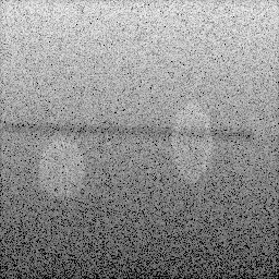
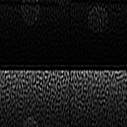
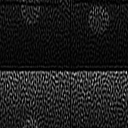
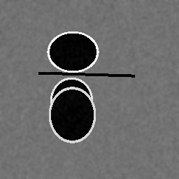
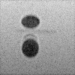
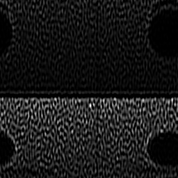
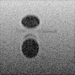
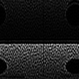
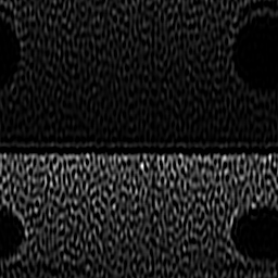
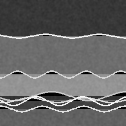
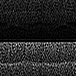
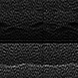
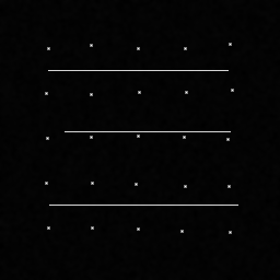
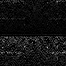
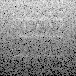
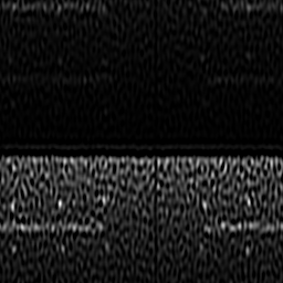
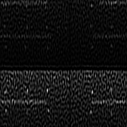
Reconstruction Gallery — 4 Scenes × 3 Scenarios
Method: CPU_baseline | Mismatch: nominal (nominal=True, perturbed=False)
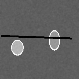
Ground Truth
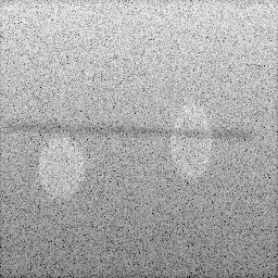
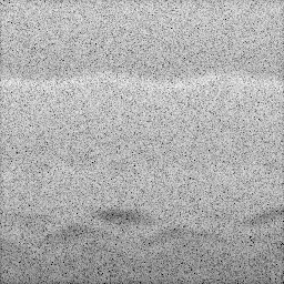
Measurement
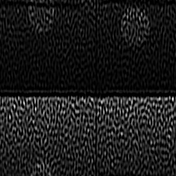
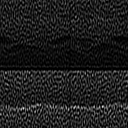
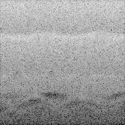
Reconstruction
Ground Truth
Measurement
Reconstruction
Ground Truth
Measurement (perturbed)
Reconstruction
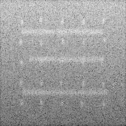
Mean PSNR Across All Scenes
Per-scene PSNR breakdown (4 scenes)
| Scene | I (PSNR) | I (SSIM) | II (PSNR) | II (SSIM) | III (PSNR) | III (SSIM) |
|---|---|---|---|---|---|---|
| scene_00 | 10.19267881704888 | 0.06760017486284199 | 9.891333366823108 | 0.08645247903796577 | 10.229768947639275 | 0.06916097429623977 |
| scene_01 | 8.618709406396592 | 0.05438400549082931 | 8.53610296730621 | 0.07716544018992613 | 8.65681449819023 | 0.0576010800630462 |
| scene_02 | 9.071305721190576 | 0.05837173538838826 | 9.608189027494609 | 0.07830817055859932 | 9.12832570289073 | 0.05927898140266334 |
| scene_03 | 18.123268932557522 | 0.2157790085948876 | 16.22729101297919 | 0.28505397170401275 | 18.130943065215487 | 0.21965784968227148 |
| Mean | 11.501490719298392 | 0.0990337310842368 | 11.06572909365078 | 0.131745015372626 | 11.536463053483931 | 0.1014247213610552 |
Experimental Setup
Key References
- Montaldo et al., 'Coherent plane-wave compounding for very high frame rate ultrasonography', IEEE TUFFC 56, 489-506 (2009)
- Liebgott et al., 'PICMUS: Plane-wave Imaging Challenge in Medical Ultrasound', IEEE IUS 2016
Canonical Datasets
- PICMUS Challenge (plane-wave ultrasound)
- CUBDL (deep learning ultrasound beamforming)
Spec DAG — Forward Model Pipeline
P(acoustic) → Σ_t → D(g, η₂)
Mismatch Parameters
| Symbol | Parameter | Description | Nominal | Perturbed |
|---|---|---|---|---|
| Δc | sos | Speed-of-sound error (m/s) | 1540 | 1560 |
| Δα | attenuation | Attenuation coefficient error (dB/cm/MHz) | 0.5 | 0.6 |
| Δs | element_sensitivity | Element sensitivity variation (%) | 0 | 5.0 |
| Δφ | phase_aberration | Phase aberration (rad) | 0 | 0.3 |
Credits System
Spec Primitives Reference (11 primitives)
Free-space or medium propagation kernel (Fresnel, Rayleigh-Sommerfeld).
Spatial or spatio-temporal amplitude modulation (coded aperture, SLM pattern).
Geometric projection operator (Radon transform, fan-beam, cone-beam).
Sampling in the Fourier / k-space domain (MRI, ptychography).
Shift-invariant convolution with a point-spread function (PSF).
Summation along a physical dimension (spectral, temporal, angular).
Sensor readout with gain g and noise model η (Gaussian, Poisson, mixed).
Patterned illumination (block, Hadamard, random) applied to the scene.
Spectral dispersion element (prism, grating) with shift α and aperture a.
Sample or gantry rotation (CT, electron tomography).
Spectral filter or monochromator selecting a wavelength band.