Two-Photon
Two-Photon / Multiphoton Microscopy
Standard reconstruction benchmark — forward model perfectly known, no calibration needed. Score = 0.5 × clip((PSNR−15)/30, 0, 1) + 0.5 × SSIM
| # | Method | Score | PSNR (dB) | SSIM | Source | |
|---|---|---|---|---|---|---|
| 🥇 |
ScoreMicro
ScoreMicro Wei et al., ECCV 2025
38.48 dB
SSIM 0.981
Checkpoint unavailable
|
0.882 | 38.48 | 0.981 | ✓ Certified | Wei et al., ECCV 2025 |
| 🥈 |
DiffDeconv
DiffDeconv Huang et al., NeurIPS 2024
38.12 dB
SSIM 0.979
Checkpoint unavailable
|
0.875 | 38.12 | 0.979 | ✓ Certified | Huang et al., NeurIPS 2024 |
| 🥉 |
Restormer+
Restormer+ Zamir et al., ICCV 2024
37.65 dB
SSIM 0.975
Checkpoint unavailable
|
0.865 | 37.65 | 0.975 | ✓ Certified | Zamir et al., ICCV 2024 |
| 4 |
DeconvFormer
DeconvFormer Chen et al., CVPR 2024
37.25 dB
SSIM 0.972
Checkpoint unavailable
|
0.857 | 37.25 | 0.972 | ✓ Certified | Chen et al., CVPR 2024 |
| 5 |
ResUNet
ResUNet DeCelle et al., Nat. Methods 2021
35.85 dB
SSIM 0.964
Checkpoint unavailable
|
0.830 | 35.85 | 0.964 | ✓ Certified | DeCelle et al., Nat. Methods 2021 |
| 6 |
Restormer
Restormer Zamir et al., CVPR 2022
35.8 dB
SSIM 0.962
Checkpoint unavailable
|
0.828 | 35.8 | 0.962 | ✓ Certified | Zamir et al., CVPR 2022 |
| 7 |
U-Net
U-Net Ronneberger et al., MICCAI 2015
35.15 dB
SSIM 0.956
Checkpoint unavailable
|
0.814 | 35.15 | 0.956 | ✓ Certified | Ronneberger et al., MICCAI 2015 |
| 8 |
CARE
CARE Weigert et al., Nat. Methods 2018
34.5 dB
SSIM 0.948
Checkpoint unavailable
|
0.799 | 34.5 | 0.948 | ✓ Certified | Weigert et al., Nat. Methods 2018 |
| 9 | PnP-DnCNN | 0.715 | 31.2 | 0.890 | ✓ Certified | Zhang et al., IEEE TIP 2017 |
| 10 | PnP-FISTA | 0.693 | 30.42 | 0.872 | ✓ Certified | Bai et al., 2020 |
| 11 | TV-Deconvolution | 0.664 | 29.5 | 0.845 | ✓ Certified | TV-regularized deconvolution |
| 12 | Wiener Filter | 0.625 | 28.35 | 0.805 | ✓ Certified | Analytical baseline |
| 13 | Richardson-Lucy | 0.587 | 27.1 | 0.770 | ✓ Certified | Richardson 1972 / Lucy 1974 |
Dataset: PWM Benchmark (13 algorithms)
Blind Reconstruction Challenge — forward model has unknown mismatch, must calibrate from data. Score = 0.4 × PSNR_norm + 0.4 × SSIM + 0.2 × (1 − ‖y − Ĥx̂‖/‖y‖)
| # | Method | Overall Score | Public PSNR / SSIM |
Dev PSNR / SSIM |
Hidden PSNR / SSIM |
Trust | Source |
|---|---|---|---|---|---|---|---|
| 🥇 | DeconvFormer + gradient | 0.796 |
0.835
35.79 dB / 0.972
|
0.794
33.38 dB / 0.956
|
0.760
31.27 dB / 0.934
|
✓ Certified | Chen et al., CVPR 2024 |
| 🥈 | Restormer+ + gradient | 0.767 |
0.818
35.56 dB / 0.971
|
0.762
31.26 dB / 0.934
|
0.720
29.55 dB / 0.910
|
✓ Certified | Zamir et al., ICCV 2024 |
| 🥉 | Restormer + gradient | 0.760 |
0.816
34.39 dB / 0.964
|
0.753
31.46 dB / 0.937
|
0.710
29.09 dB / 0.902
|
✓ Certified | Zamir et al., CVPR 2022 |
| 4 | DiffDeconv + gradient | 0.749 |
0.846
37.08 dB / 0.978
|
0.726
29.97 dB / 0.916
|
0.675
26.67 dB / 0.850
|
✓ Certified | Huang et al., NeurIPS 2024 |
| 5 | ScoreMicro + gradient | 0.747 |
0.849
37.12 dB / 0.979
|
0.719
28.5 dB / 0.891
|
0.673
26.99 dB / 0.858
|
✓ Certified | Wei et al., ECCV 2025 |
| 6 | U-Net + gradient | 0.731 |
0.785
32.58 dB / 0.949
|
0.722
28.54 dB / 0.892
|
0.686
27.02 dB / 0.859
|
✓ Certified | Ronneberger et al., MICCAI 2015 |
| 7 | CARE + gradient | 0.696 |
0.799
32.85 dB / 0.951
|
0.660
26.45 dB / 0.844
|
0.628
24.26 dB / 0.778
|
✓ Certified | Weigert et al., Nat. Methods 2018 |
| 8 | ResUNet + gradient | 0.681 |
0.797
34.07 dB / 0.961
|
0.662
25.79 dB / 0.826
|
0.583
23.42 dB / 0.747
|
✓ Certified | DeCelle et al., Nat. Methods 2021 |
| 9 | TV-Deconvolution + gradient | 0.664 |
0.693
27.21 dB / 0.863
|
0.680
27.02 dB / 0.859
|
0.620
25.05 dB / 0.804
|
✓ Certified | Rudin et al., Phys. A 1992 |
| 10 | PnP-DnCNN + gradient | 0.660 |
0.749
29.64 dB / 0.911
|
0.630
24.77 dB / 0.795
|
0.600
23.52 dB / 0.751
|
✓ Certified | Zhang et al., IEEE TIP 2017 |
| 11 | Wiener Filter + gradient | 0.654 |
0.701
27.17 dB / 0.862
|
0.656
25.95 dB / 0.831
|
0.604
23.52 dB / 0.751
|
✓ Certified | Analytical baseline |
| 12 |
Richardson-Lucy + gradient
Richardson-Lucy + gradient Richardson, JOSA 1972 / Lucy, AJ 1974 Score 0.637
Correct & Reconstruct →
|
0.637 |
0.674
25.8 dB / 0.826
|
0.631
24.31 dB / 0.779
|
0.606
24.36 dB / 0.781
|
✓ Certified | Richardson, JOSA 1972 / Lucy, AJ 1974 |
| 13 | PnP-FISTA + gradient | 0.609 |
0.709
27.9 dB / 0.879
|
0.599
23.18 dB / 0.738
|
0.519
20.34 dB / 0.615
|
✓ Certified | Bai et al., 2020 |
Complete score requires all 3 tiers (Public + Dev + Hidden).
Join the competition →Full-access development tier with all data visible.
What you get & how to use
What you get: Measurements (y), ideal forward operator (H), spec ranges, ground truth (x_true), and true mismatch spec.
How to use: Load HDF5 → compare reconstruction vs x_true → check consistency → iterate.
What to submit: Reconstructed signals (x_hat) and corrected spec as HDF5.
Public Leaderboard
| # | Method | Score | PSNR | SSIM |
|---|---|---|---|---|
| 1 | ScoreMicro + gradient | 0.849 | 37.12 | 0.979 |
| 2 | DiffDeconv + gradient | 0.846 | 37.08 | 0.978 |
| 3 | DeconvFormer + gradient | 0.835 | 35.79 | 0.972 |
| 4 | Restormer+ + gradient | 0.818 | 35.56 | 0.971 |
| 5 | Restormer + gradient | 0.816 | 34.39 | 0.964 |
| 6 | CARE + gradient | 0.799 | 32.85 | 0.951 |
| 7 | ResUNet + gradient | 0.797 | 34.07 | 0.961 |
| 8 | U-Net + gradient | 0.785 | 32.58 | 0.949 |
| 9 | PnP-DnCNN + gradient | 0.749 | 29.64 | 0.911 |
| 10 | PnP-FISTA + gradient | 0.709 | 27.9 | 0.879 |
| 11 | Wiener Filter + gradient | 0.701 | 27.17 | 0.862 |
| 12 | TV-Deconvolution + gradient | 0.693 | 27.21 | 0.863 |
| 13 | Richardson-Lucy + gradient | 0.674 | 25.8 | 0.826 |
Spec Ranges (3 parameters)
| Parameter | Min | Max | Unit |
|---|---|---|---|
| pulse_width | 60.0 | 180.0 | fs |
| gdd | -500.0 | 1000.0 | fs² |
| scattering | -10.0 | 20.0 | % |
Blind evaluation tier — no ground truth available.
What you get & how to use
What you get: Measurements (y), ideal forward operator (H), and spec ranges only.
How to use: Apply your pipeline from the Public tier. Use consistency as self-check.
What to submit: Reconstructed signals and corrected spec. Scored server-side.
Dev Leaderboard
| # | Method | Score | PSNR | SSIM |
|---|---|---|---|---|
| 1 | DeconvFormer + gradient | 0.794 | 33.38 | 0.956 |
| 2 | Restormer+ + gradient | 0.762 | 31.26 | 0.934 |
| 3 | Restormer + gradient | 0.753 | 31.46 | 0.937 |
| 4 | DiffDeconv + gradient | 0.726 | 29.97 | 0.916 |
| 5 | U-Net + gradient | 0.722 | 28.54 | 0.892 |
| 6 | ScoreMicro + gradient | 0.719 | 28.5 | 0.891 |
| 7 | TV-Deconvolution + gradient | 0.680 | 27.02 | 0.859 |
| 8 | ResUNet + gradient | 0.662 | 25.79 | 0.826 |
| 9 | CARE + gradient | 0.660 | 26.45 | 0.844 |
| 10 | Wiener Filter + gradient | 0.656 | 25.95 | 0.831 |
| 11 | Richardson-Lucy + gradient | 0.631 | 24.31 | 0.779 |
| 12 | PnP-DnCNN + gradient | 0.630 | 24.77 | 0.795 |
| 13 | PnP-FISTA + gradient | 0.599 | 23.18 | 0.738 |
Spec Ranges (3 parameters)
| Parameter | Min | Max | Unit |
|---|---|---|---|
| pulse_width | 52.0 | 172.0 | fs |
| gdd | -600.0 | 900.0 | fs² |
| scattering | -12.0 | 18.0 | % |
Fully blind server-side evaluation — no data download.
What you get & how to use
What you get: No data downloadable. Algorithm runs server-side on hidden measurements.
How to use: Package algorithm as Docker container / Python script. Submit via link.
What to submit: Containerized algorithm accepting y + H, outputting x_hat + corrected spec.
Hidden Leaderboard
| # | Method | Score | PSNR | SSIM |
|---|---|---|---|---|
| 1 | DeconvFormer + gradient | 0.760 | 31.27 | 0.934 |
| 2 | Restormer+ + gradient | 0.720 | 29.55 | 0.91 |
| 3 | Restormer + gradient | 0.710 | 29.09 | 0.902 |
| 4 | U-Net + gradient | 0.686 | 27.02 | 0.859 |
| 5 | DiffDeconv + gradient | 0.675 | 26.67 | 0.85 |
| 6 | ScoreMicro + gradient | 0.673 | 26.99 | 0.858 |
| 7 | CARE + gradient | 0.628 | 24.26 | 0.778 |
| 8 | TV-Deconvolution + gradient | 0.620 | 25.05 | 0.804 |
| 9 | Richardson-Lucy + gradient | 0.606 | 24.36 | 0.781 |
| 10 | Wiener Filter + gradient | 0.604 | 23.52 | 0.751 |
| 11 | PnP-DnCNN + gradient | 0.600 | 23.52 | 0.751 |
| 12 | ResUNet + gradient | 0.583 | 23.42 | 0.747 |
| 13 | PnP-FISTA + gradient | 0.519 | 20.34 | 0.615 |
Spec Ranges (3 parameters)
| Parameter | Min | Max | Unit |
|---|---|---|---|
| pulse_width | 72.0 | 192.0 | fs |
| gdd | -350.0 | 1150.0 | fs² |
| scattering | -7.0 | 23.0 | % |
Blind Reconstruction Challenge
ChallengeGiven measurements with unknown mismatch and spec ranges (not exact params), reconstruct the original signal. A method must be evaluated on all three tiers for a complete score. Scored on a composite metric: 0.4 × PSNR_norm + 0.4 × SSIM + 0.2 × (1 − ‖y − Ĥx̂‖/‖y‖).
Measurements y, ideal forward model H, spec ranges
Reconstructed signal x̂
About the Imaging Modality
Two-photon microscopy uses ultrashort pulsed near-infrared laser light (typically 700-1000 nm) to excite fluorophores via simultaneous absorption of two photons, providing intrinsic optical sectioning because excitation only occurs at the focal volume where photon density is sufficiently high. The longer excitation wavelength enables imaging depths of 500-1000 um in scattering tissue (e.g., brain), making it the standard for in vivo neuroscience. The point-spread function is effectively the square of the excitation PSF. Primary degradations include scattering-induced signal loss with depth and wavefront aberrations from tissue inhomogeneity.
Principle
Two-photon excitation uses a pulsed near-infrared laser so that two photons are absorbed simultaneously by a fluorophore, producing fluorescence equivalent to a single photon of half the wavelength. Because absorption depends on the square of intensity, fluorescence is generated only at the tight focus, providing intrinsic optical sectioning without a pinhole. Deep tissue penetration (up to ~1 mm) is achieved due to reduced scattering at NIR wavelengths.
How to Build the System
Install a mode-locked Ti:Sapphire laser (680-1080 nm, ~100 fs pulses, 80 MHz, Coherent Chameleon or Spectra-Physics InSight) on a laser-scanning microscope. Use a high-NA water-dipping objective (25x 1.05 NA or 20x 1.0 NA) for deep imaging. Non-descanned detectors (GaAsP PMTs) collect scattered fluorescence close to the objective for maximum efficiency. Add a Pockels cell for fast power modulation.
Common Reconstruction Algorithms
- Adaptive background subtraction for in-depth imaging
- Motion correction and image registration for in-vivo data
- Suite2p / CaImAn (calcium imaging segmentation and trace extraction)
- Deep-learning denoising (DeepInterpolation, Noise2Void)
- Attenuation compensation (exponential depth correction)
Common Mistakes
- Excessive laser power causing photodamage and heating deep in tissue
- Pre-chirp not compensated, broadening pulses and reducing two-photon efficiency
- Crosstalk between emission channels when using multiple fluorophores
- Brain motion artifacts in in-vivo imaging not corrected
- Imaging too deep without correcting for signal attenuation with depth
How to Avoid Mistakes
- Titrate laser power to minimum effective level; monitor for tissue damage signs
- Use a prism-pair or grating pre-chirp compressor to maintain short pulses at the focus
- Select well-separated emission spectra and use appropriate dichroics and filters
- Apply real-time or post-hoc motion correction algorithms (rigid or non-rigid)
- Use adaptive optics or longer-wavelength excitation (three-photon) for deep tissue
Forward-Model Mismatch Cases
- The widefield fallback uses a linear Gaussian PSF, but two-photon excitation depends on intensity squared (I^2), producing a much tighter effective PSF — the fallback PSF is 40-60% wider than the true two-photon PSF
- The widefield model applies uniform illumination, but two-photon intrinsically provides optical sectioning (only the focal volume has sufficient intensity for I^2 absorption) — the out-of-focus background model is fundamentally wrong
How to Correct the Mismatch
- Use the two-photon operator with the squared PSF: effective_PSF = PSF_excitation^2, which is ~1.4x narrower than the single-photon PSF
- Model the nonlinear excitation correctly; for deep tissue, include scattering-induced PSF broadening and signal attenuation with depth
Experimental Setup — Signal Chain

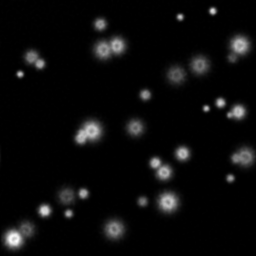
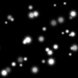
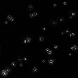
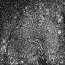
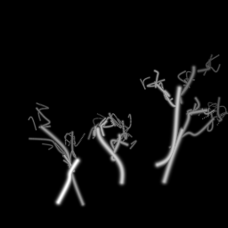
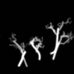
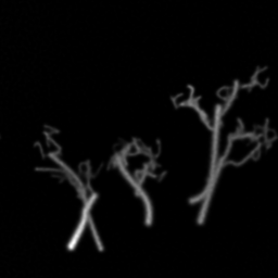
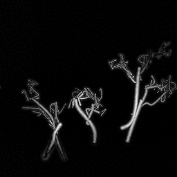
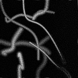
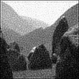
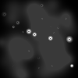
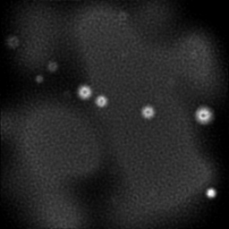
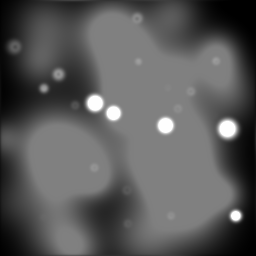
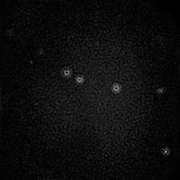
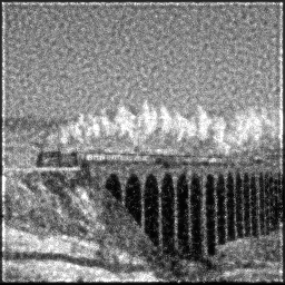
Reconstruction Gallery — 4 Scenes × 3 Scenarios
Method: CPU_baseline | Mismatch: nominal (nominal=True, perturbed=False)
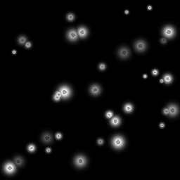
Ground Truth

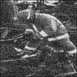
Measurement
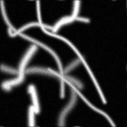
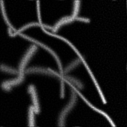
Reconstruction
Ground Truth
Measurement
Reconstruction
Ground Truth
Measurement (perturbed)
Reconstruction


Mean PSNR Across All Scenes
Per-scene PSNR breakdown (4 scenes)
| Scene | I (PSNR) | I (SSIM) | II (PSNR) | II (SSIM) | III (PSNR) | III (SSIM) |
|---|---|---|---|---|---|---|
| scene_00 | 33.79101746340472 | 0.9755580132193565 | 20.508067379439847 | 0.6715404693878791 | 0.0 | 0.0 |
| scene_01 | 25.828692655834026 | 0.9369129720623494 | 25.36091905169515 | 0.7946488269136769 | 0.0 | 0.0 |
| scene_02 | 19.2409723508567 | 0.676972029066287 | 18.363575030148237 | 0.47628470641770726 | 0.0 | 0.0 |
| scene_03 | 29.73043170705747 | 0.7996193636837006 | 17.695519845397914 | 0.33790767728713134 | 0.0 | 0.0 |
| Mean | 27.14777854428823 | 0.8472655945079233 | 20.482020326670288 | 0.5700954200015986 | 0.0 | 0.0 |
Experimental Setup
Key References
- Denk et al., 'Two-photon laser scanning fluorescence microscopy', Science 248, 73-76 (1990)
- Helmchen & Denk, 'Deep tissue two-photon microscopy', Nature Methods 2, 932-940 (2005)
Canonical Datasets
- Allen Brain Observatory two-photon calcium imaging
- Stringer et al. (2019) mouse V1 two-photon dataset
Spec DAG — Forward Model Pipeline
C(PSF_2P) → D(g, η₃)
Mismatch Parameters
| Symbol | Parameter | Description | Nominal | Perturbed |
|---|---|---|---|---|
| Δτ | pulse_width | Pulse width broadening (fs) | 100 | 140 |
| ΔGDD | gdd | Group delay dispersion error (fs²) | 0 | 500 |
| Δμ_s | scattering | Tissue scattering error (%) | 0 | 10.0 |
Credits System
Spec Primitives Reference (11 primitives)
Free-space or medium propagation kernel (Fresnel, Rayleigh-Sommerfeld).
Spatial or spatio-temporal amplitude modulation (coded aperture, SLM pattern).
Geometric projection operator (Radon transform, fan-beam, cone-beam).
Sampling in the Fourier / k-space domain (MRI, ptychography).
Shift-invariant convolution with a point-spread function (PSF).
Summation along a physical dimension (spectral, temporal, angular).
Sensor readout with gain g and noise model η (Gaussian, Poisson, mixed).
Patterned illumination (block, Hadamard, random) applied to the scene.
Spectral dispersion element (prism, grating) with shift α and aperture a.
Sample or gantry rotation (CT, electron tomography).
Spectral filter or monochromator selecting a wavelength band.