ToF Camera
Time-of-Flight Depth Camera
Standard reconstruction benchmark — forward model perfectly known, no calibration needed. Score = 0.5 × clip((PSNR−15)/30, 0, 1) + 0.5 × SSIM
| # | Method | Score | PSNR (dB) | SSIM | Source | |
|---|---|---|---|---|---|---|
| 🥇 |
MPI-Former
MPI-Former Multi-path interference correction, 2023
34.0 dB
SSIM 0.930
Checkpoint unavailable
|
0.782 | 34.0 | 0.930 | ✓ Certified | Multi-path interference correction, 2023 |
| 🥈 |
DeepToF
DeepToF Marco et al., ECCV 2018
32.5 dB
SSIM 0.900
Checkpoint unavailable
|
0.742 | 32.5 | 0.900 | ✓ Certified | Marco et al., ECCV 2018 |
| 🥉 | PnP-ToF | 0.617 | 28.0 | 0.800 | ✓ Certified | PnP with depth prior for ToF |
| 4 | Phase Unwrap | 0.480 | 24.0 | 0.660 | ✓ Certified | Bamji et al., IEEE SSC 2015 |
Dataset: PWM Benchmark (4 algorithms)
Blind Reconstruction Challenge — forward model has unknown mismatch, must calibrate from data. Score = 0.4 × PSNR_norm + 0.4 × SSIM + 0.2 × (1 − ‖y − Ĥx̂‖/‖y‖)
| # | Method | Overall Score | Public PSNR / SSIM |
Dev PSNR / SSIM |
Hidden PSNR / SSIM |
Trust | Source |
|---|---|---|---|---|---|---|---|
| 🥇 | MPI-Former + gradient | 0.677 |
0.768
31.5 dB / 0.937
|
0.685
26.89 dB / 0.855
|
0.578
22.36 dB / 0.705
|
✓ Certified | Multi-path interference correction, 2023 |
| 🥈 | DeepToF + gradient | 0.664 |
0.749
30.66 dB / 0.926
|
0.643
24.84 dB / 0.797
|
0.599
23.17 dB / 0.738
|
✓ Certified | Marco et al., ECCV 2018 |
| 🥉 | PnP-ToF + gradient | 0.614 |
0.690
26.46 dB / 0.844
|
0.587
22.71 dB / 0.720
|
0.564
21.85 dB / 0.684
|
✓ Certified | PnP with depth prior for ToF |
| 4 | Phase Unwrap + gradient | 0.517 |
0.595
22.42 dB / 0.708
|
0.508
19.73 dB / 0.586
|
0.448
17.92 dB / 0.496
|
✓ Certified | Bamji et al., IEEE SSC 2015 |
Complete score requires all 3 tiers (Public + Dev + Hidden).
Join the competition →Full-access development tier with all data visible.
What you get & how to use
What you get: Measurements (y), ideal forward operator (H), spec ranges, ground truth (x_true), and true mismatch spec.
How to use: Load HDF5 → compare reconstruction vs x_true → check consistency → iterate.
What to submit: Reconstructed signals (x_hat) and corrected spec as HDF5.
Public Leaderboard
| # | Method | Score | PSNR | SSIM |
|---|---|---|---|---|
| 1 | MPI-Former + gradient | 0.768 | 31.5 | 0.937 |
| 2 | DeepToF + gradient | 0.749 | 30.66 | 0.926 |
| 3 | PnP-ToF + gradient | 0.690 | 26.46 | 0.844 |
| 4 | Phase Unwrap + gradient | 0.595 | 22.42 | 0.708 |
Spec Ranges (3 parameters)
| Parameter | Min | Max | Unit |
|---|---|---|---|
| modulation_freq | 19.9 | 20.2 | MHz |
| multipath | -5.0 | 10.0 | % |
| phase_nonlinearity | -2.0 | 4.0 | deg |
Blind evaluation tier — no ground truth available.
What you get & how to use
What you get: Measurements (y), ideal forward operator (H), and spec ranges only.
How to use: Apply your pipeline from the Public tier. Use consistency as self-check.
What to submit: Reconstructed signals and corrected spec. Scored server-side.
Dev Leaderboard
| # | Method | Score | PSNR | SSIM |
|---|---|---|---|---|
| 1 | MPI-Former + gradient | 0.685 | 26.89 | 0.855 |
| 2 | DeepToF + gradient | 0.643 | 24.84 | 0.797 |
| 3 | PnP-ToF + gradient | 0.587 | 22.71 | 0.72 |
| 4 | Phase Unwrap + gradient | 0.508 | 19.73 | 0.586 |
Spec Ranges (3 parameters)
| Parameter | Min | Max | Unit |
|---|---|---|---|
| modulation_freq | 19.88 | 20.18 | MHz |
| multipath | -6.0 | 9.0 | % |
| phase_nonlinearity | -2.4 | 3.6 | deg |
Fully blind server-side evaluation — no data download.
What you get & how to use
What you get: No data downloadable. Algorithm runs server-side on hidden measurements.
How to use: Package algorithm as Docker container / Python script. Submit via link.
What to submit: Containerized algorithm accepting y + H, outputting x_hat + corrected spec.
Hidden Leaderboard
| # | Method | Score | PSNR | SSIM |
|---|---|---|---|---|
| 1 | DeepToF + gradient | 0.599 | 23.17 | 0.738 |
| 2 | MPI-Former + gradient | 0.578 | 22.36 | 0.705 |
| 3 | PnP-ToF + gradient | 0.564 | 21.85 | 0.684 |
| 4 | Phase Unwrap + gradient | 0.448 | 17.92 | 0.496 |
Spec Ranges (3 parameters)
| Parameter | Min | Max | Unit |
|---|---|---|---|
| modulation_freq | 19.93 | 20.23 | MHz |
| multipath | -3.5 | 11.5 | % |
| phase_nonlinearity | -1.4 | 4.6 | deg |
Blind Reconstruction Challenge
ChallengeGiven measurements with unknown mismatch and spec ranges (not exact params), reconstruct the original signal. A method must be evaluated on all three tiers for a complete score. Scored on a composite metric: 0.4 × PSNR_norm + 0.4 × SSIM + 0.2 × (1 − ‖y − Ĥx̂‖/‖y‖).
Measurements y, ideal forward model H, spec ranges
Reconstructed signal x̂
About the Imaging Modality
ToF cameras measure per-pixel depth by emitting modulated near-infrared light and measuring the phase delay of the reflected signal relative to the emitted signal. In amplitude-modulated continuous-wave (AMCW) ToF, the phase offset phi = 2*pi*f*2d/c encodes the round-trip distance 2d. Multiple modulation frequencies resolve depth ambiguity. Primary degradations include multi-path interference (MPI), motion blur, and systematic errors at depth discontinuities (flying pixels).
Principle
A Time-of-Flight depth camera measures the round-trip time of modulated light (typically near-infrared LEDs at 850 nm) reflected from the scene. The sensor measures the phase shift between emitted and received modulated signals at each pixel, which is proportional to the target distance: d = c·Δφ/(4π·f_mod). Typical modulation frequencies are 20-100 MHz, providing depth ranges of 0.5-10 meters with mm-cm precision.
How to Build the System
Use an integrated ToF camera module (e.g., Microsoft Azure Kinect DK, PMD CamBoard pico, Texas Instruments OPT8241). The module contains the NIR light source, modulation driver, and ToF sensor with per-pixel demodulation circuits. Mount rigidly and calibrate intrinsic parameters (lens distortion, depth offset) and phase-to-depth nonlinearities. For multi-camera setups, synchronize or frequency-multiplex to avoid interference.
Common Reconstruction Algorithms
- Four-phase demodulation for distance extraction
- Multi-frequency unwrapping for extended unambiguous range
- Flying-pixel filtering (mixed pixels at depth discontinuities)
- Multi-path interference correction
- Deep-learning depth denoising and completion
Common Mistakes
- Multi-path interference causing systematic depth errors in concave scenes
- Flying pixels at depth edges producing incorrect intermediate depth values
- Phase wrapping ambiguity when objects exceed the unambiguous range
- Interference from ambient NIR light (sunlight) degrading outdoor performance
- Systematic depth errors from non-ideal sensor response not calibrated out
How to Avoid Mistakes
- Use multi-path correction algorithms or multi-frequency modulation
- Apply flying-pixel detection and removal based on amplitude and neighbor consistency
- Use dual-frequency operation to extend the unambiguous range
- Use narrow-band optical filter and higher modulation power for outdoor use
- Perform per-pixel depth calibration with a known flat reference at multiple distances
Forward-Model Mismatch Cases
- The widefield fallback produces a 2D intensity image, but ToF cameras measure depth via phase shift of modulated near-infrared light — the distance information (d = c*dphi/(4*pi*f_mod)) is entirely absent from the blurred image
- ToF measurement involves demodulation of the reflected modulated signal at each pixel, producing amplitude, phase, and confidence maps — the widefield intensity-only blur cannot produce depth or distinguish multi-path interference
How to Correct the Mismatch
- Use the ToF camera operator that models modulated illumination and per-pixel demodulation: four-phase sampling extracts the phase shift proportional to target distance at each pixel
- Apply phase-to-depth conversion, multi-path correction, and flying-pixel filtering using the correct modulation frequency, amplitude, and phase measurement model
Experimental Setup — Signal Chain

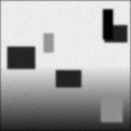
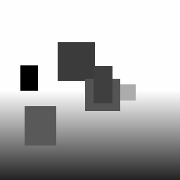
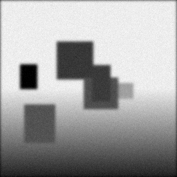
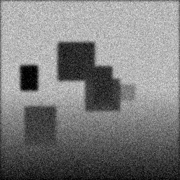
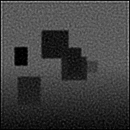
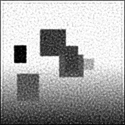
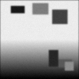
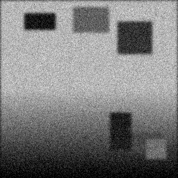
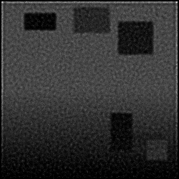
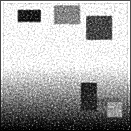
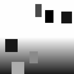
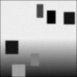
Reconstruction Gallery — 4 Scenes × 3 Scenarios
Method: CPU_baseline | Mismatch: nominal (nominal=True, perturbed=False)

Ground Truth
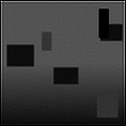
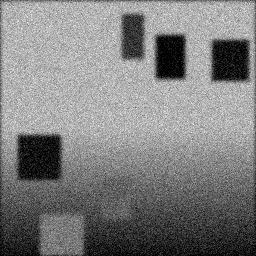
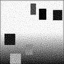
Measurement
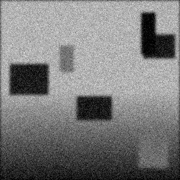
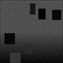
Reconstruction
Ground Truth
Measurement
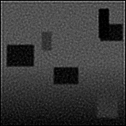
Reconstruction
Ground Truth
Measurement (perturbed)
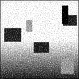
Reconstruction


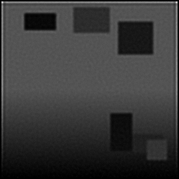

Mean PSNR Across All Scenes
Per-scene PSNR breakdown (4 scenes)
| Scene | I (PSNR) | I (SSIM) | II (PSNR) | II (SSIM) | III (PSNR) | III (SSIM) |
|---|---|---|---|---|---|---|
| scene_00 | 5.527214497768322 | 0.4672006439363062 | 5.459345679167983 | 0.19945611529107565 | 18.401943105213206 | 0.2341331320438871 |
| scene_01 | 5.806026384875609 | 0.4796046249826327 | 6.030423203911414 | 0.19344004863131214 | 18.47044552189445 | 0.22669922821491817 |
| scene_02 | 5.6571772261462066 | 0.46600075432368365 | 5.076086325487175 | 0.20923461502441765 | 18.605513677538003 | 0.23724583293967508 |
| scene_03 | 5.389777474892018 | 0.468956853362985 | 5.2322280218118955 | 0.2040550582761015 | 18.40005847928955 | 0.2386520108290784 |
| Mean | 5.595048895920539 | 0.47044071915140184 | 5.449520807594617 | 0.20154645930572673 | 18.469490195983802 | 0.23418255100688967 |
Experimental Setup
Key References
- Hansard et al., 'Time-of-Flight Cameras: Principles, Methods and Applications', Springer (2013)
Canonical Datasets
- NYU Depth V2 (Silberman et al.)
- KITTI depth benchmark (adapted)
Spec DAG — Forward Model Pipeline
P(modulated) → Σ(correlation) → D(g, η₁)
Mismatch Parameters
| Symbol | Parameter | Description | Nominal | Perturbed |
|---|---|---|---|---|
| Δf_m | modulation_freq | Modulation frequency error (MHz) | 20 | 20.1 |
| I_mp | multipath | Multipath interference intensity (%) | 0 | 5.0 |
| Δφ | phase_nonlinearity | Phase nonlinearity (deg) | 0 | 2.0 |
Credits System
Spec Primitives Reference (11 primitives)
Free-space or medium propagation kernel (Fresnel, Rayleigh-Sommerfeld).
Spatial or spatio-temporal amplitude modulation (coded aperture, SLM pattern).
Geometric projection operator (Radon transform, fan-beam, cone-beam).
Sampling in the Fourier / k-space domain (MRI, ptychography).
Shift-invariant convolution with a point-spread function (PSF).
Summation along a physical dimension (spectral, temporal, angular).
Sensor readout with gain g and noise model η (Gaussian, Poisson, mixed).
Patterned illumination (block, Hadamard, random) applied to the scene.
Spectral dispersion element (prism, grating) with shift α and aperture a.
Sample or gantry rotation (CT, electron tomography).
Spectral filter or monochromator selecting a wavelength band.