SAR
Synthetic Aperture Radar
Standard reconstruction benchmark — forward model perfectly known, no calibration needed. Score = 0.5 × clip((PSNR−15)/30, 0, 1) + 0.5 × SSIM
| # | Method | Score | PSNR (dB) | SSIM | Source | |
|---|---|---|---|---|---|---|
| 🥇 |
DiffusionSAR
DiffusionSAR Wei et al., NeurIPS 2024
35.42 dB
SSIM 0.955
Checkpoint unavailable
|
0.818 | 35.42 | 0.955 | ✓ Certified | Wei et al., NeurIPS 2024 |
| 🥈 |
PanSharpener++
PanSharpener++ Zhang et al., ICCV 2024
34.58 dB
SSIM 0.945
Checkpoint unavailable
|
0.799 | 34.58 | 0.945 | ✓ Certified | Zhang et al., ICCV 2024 |
| 🥉 |
SARFormer
SARFormer Li et al., CVPR 2024
33.85 dB
SSIM 0.932
Checkpoint unavailable
|
0.780 | 33.85 | 0.932 | ✓ Certified | Li et al., CVPR 2024 |
| 4 |
ScoreSAR
ScoreSAR Johnson et al., ECCV 2025
31.9 dB
SSIM 0.942
Checkpoint unavailable
|
0.753 | 31.9 | 0.942 | ✓ Certified | Johnson et al., ECCV 2025 |
| 5 |
SAR-CAM
SAR-CAM Cross-attention SAR, 2024
32.1 dB
SSIM 0.912
Checkpoint unavailable
|
0.741 | 32.1 | 0.912 | ✓ Certified | Cross-attention SAR, 2024 |
| 6 |
SARDenoiserViT
SARDenoiserViT Wang et al., ICCV 2024
30.2 dB
SSIM 0.920
Checkpoint unavailable
|
0.713 | 30.2 | 0.920 | ✓ Certified | Wang et al., ICCV 2024 |
| 7 |
SAR-DRN
SAR-DRN Zhang et al., RS 2018
30.6 dB
SSIM 0.882
Checkpoint unavailable
|
0.701 | 30.6 | 0.882 | ✓ Certified | Zhang et al., RS 2018 |
| 8 |
SAR-ResNet
SAR-ResNet Chen et al., IEEE TGRS 2022
28.84 dB
SSIM 0.897
Checkpoint unavailable
|
0.679 | 28.84 | 0.897 | ✓ Certified | Chen et al., IEEE TGRS 2022 |
| 9 | Lee Filter | 0.677 | 28.75 | 0.896 | ✓ Certified | Lee, IEEE TGRS 1980 |
| 10 | SAR-BM3D | 0.598 | 27.2 | 0.790 | ✓ Certified | Parrilli et al., IEEE TGRS 2012 |
| 11 | Range-Doppler | 0.596 | 25.9 | 0.829 | ✓ Certified | SAR signal processing baseline |
| 12 | Chirp Scaling | 0.487 | 22.68 | 0.718 | ✓ Certified | Raney et al., IEEE TGRS 1994 |
| 13 | Matched Filter | 0.462 | 23.5 | 0.640 | ✓ Certified | Standard SAR focusing |
Dataset: PWM Benchmark (13 algorithms)
Blind Reconstruction Challenge — forward model has unknown mismatch, must calibrate from data. Score = 0.4 × PSNR_norm + 0.4 × SSIM + 0.2 × (1 − ‖y − Ĥx̂‖/‖y‖)
| # | Method | Overall Score | Public PSNR / SSIM |
Dev PSNR / SSIM |
Hidden PSNR / SSIM |
Trust | Source |
|---|---|---|---|---|---|---|---|
| 🥇 | DiffusionSAR + gradient | 0.731 |
0.789
33.01 dB / 0.953
|
0.729
29.75 dB / 0.913
|
0.676
27.68 dB / 0.874
|
✓ Certified | Wei et al., NeurIPS 2024 |
| 🥈 | SARFormer + gradient | 0.693 |
0.762
30.88 dB / 0.929
|
0.690
26.85 dB / 0.854
|
0.626
24.88 dB / 0.798
|
✓ Certified | Li et al., CVPR 2024 |
| 🥉 | SAR-CAM + gradient | 0.689 |
0.738
29.47 dB / 0.908
|
0.704
28.2 dB / 0.885
|
0.624
24.86 dB / 0.798
|
✓ Certified | Cross-attention SAR, 2024 |
| 4 | PanSharpener++ + gradient | 0.669 |
0.803
33.58 dB / 0.958
|
0.654
25.7 dB / 0.823
|
0.551
21.32 dB / 0.660
|
✓ Certified | Zhang et al., ICCV 2024 |
| 5 | ScoreSAR + gradient | 0.647 |
0.732
28.9 dB / 0.898
|
0.627
24.14 dB / 0.773
|
0.582
23.23 dB / 0.740
|
✓ Certified | Johnson et al., ECCV 2025 |
| 6 | Lee Filter + gradient | 0.646 |
0.705
27.18 dB / 0.862
|
0.626
24.87 dB / 0.798
|
0.607
24.07 dB / 0.771
|
✓ Certified | Lee, IEEE TGRS 1980 |
| 7 | SAR-DRN + gradient | 0.621 |
0.717
28.46 dB / 0.890
|
0.617
24.23 dB / 0.777
|
0.529
20.68 dB / 0.631
|
✓ Certified | Zhang et al., RS 2018 |
| 8 | Range-Doppler + gradient | 0.610 |
0.617
23.74 dB / 0.759
|
0.613
23.97 dB / 0.767
|
0.600
23.52 dB / 0.751
|
✓ Certified | SAR signal processing baseline |
| 9 | SARDenoiserViT + gradient | 0.609 |
0.732
28.51 dB / 0.891
|
0.606
24.03 dB / 0.770
|
0.488
19.33 dB / 0.566
|
✓ Certified | Wang et al., ICCV 2024 |
| 10 | SAR-ResNet + gradient | 0.596 |
0.708
27.36 dB / 0.867
|
0.572
22.08 dB / 0.693
|
0.508
20.7 dB / 0.632
|
✓ Certified | Chen et al., IEEE TGRS 2022 |
| 11 | SAR-BM3D + gradient | 0.572 |
0.645
24.9 dB / 0.799
|
0.555
21.54 dB / 0.670
|
0.516
20.28 dB / 0.612
|
✓ Certified | Parrilli et al., IEEE TGRS 2012 |
| 12 | Chirp Scaling + gradient | 0.509 |
0.558
21.01 dB / 0.646
|
0.495
19.98 dB / 0.598
|
0.473
19.44 dB / 0.572
|
✓ Certified | Raney et al., IEEE TGRS 1994 |
| 13 | Matched Filter + gradient | 0.496 |
0.542
20.79 dB / 0.636
|
0.499
19.98 dB / 0.598
|
0.447
18.38 dB / 0.519
|
✓ Certified | Standard SAR focusing |
Complete score requires all 3 tiers (Public + Dev + Hidden).
Join the competition →Full-access development tier with all data visible.
What you get & how to use
What you get: Measurements (y), ideal forward operator (H), spec ranges, ground truth (x_true), and true mismatch spec.
How to use: Load HDF5 → compare reconstruction vs x_true → check consistency → iterate.
What to submit: Reconstructed signals (x_hat) and corrected spec as HDF5.
Public Leaderboard
| # | Method | Score | PSNR | SSIM |
|---|---|---|---|---|
| 1 | PanSharpener++ + gradient | 0.803 | 33.58 | 0.958 |
| 2 | DiffusionSAR + gradient | 0.789 | 33.01 | 0.953 |
| 3 | SARFormer + gradient | 0.762 | 30.88 | 0.929 |
| 4 | SAR-CAM + gradient | 0.738 | 29.47 | 0.908 |
| 5 | ScoreSAR + gradient | 0.732 | 28.9 | 0.898 |
| 6 | SARDenoiserViT + gradient | 0.732 | 28.51 | 0.891 |
| 7 | SAR-DRN + gradient | 0.717 | 28.46 | 0.89 |
| 8 | SAR-ResNet + gradient | 0.708 | 27.36 | 0.867 |
| 9 | Lee Filter + gradient | 0.705 | 27.18 | 0.862 |
| 10 | SAR-BM3D + gradient | 0.645 | 24.9 | 0.799 |
| 11 | Range-Doppler + gradient | 0.617 | 23.74 | 0.759 |
| 12 | Chirp Scaling + gradient | 0.558 | 21.01 | 0.646 |
| 13 | Matched Filter + gradient | 0.542 | 20.79 | 0.636 |
Spec Ranges (3 parameters)
| Parameter | Min | Max | Unit |
|---|---|---|---|
| motion_error | -2.0 | 4.0 | cm |
| phase_error | -0.3 | 0.6 | rad |
| range_cell_migration | -0.5 | 1.0 | cells |
Blind evaluation tier — no ground truth available.
What you get & how to use
What you get: Measurements (y), ideal forward operator (H), and spec ranges only.
How to use: Apply your pipeline from the Public tier. Use consistency as self-check.
What to submit: Reconstructed signals and corrected spec. Scored server-side.
Dev Leaderboard
| # | Method | Score | PSNR | SSIM |
|---|---|---|---|---|
| 1 | DiffusionSAR + gradient | 0.729 | 29.75 | 0.913 |
| 2 | SAR-CAM + gradient | 0.704 | 28.2 | 0.885 |
| 3 | SARFormer + gradient | 0.690 | 26.85 | 0.854 |
| 4 | PanSharpener++ + gradient | 0.654 | 25.7 | 0.823 |
| 5 | ScoreSAR + gradient | 0.627 | 24.14 | 0.773 |
| 6 | Lee Filter + gradient | 0.626 | 24.87 | 0.798 |
| 7 | SAR-DRN + gradient | 0.617 | 24.23 | 0.777 |
| 8 | Range-Doppler + gradient | 0.613 | 23.97 | 0.767 |
| 9 | SARDenoiserViT + gradient | 0.606 | 24.03 | 0.77 |
| 10 | SAR-ResNet + gradient | 0.572 | 22.08 | 0.693 |
| 11 | SAR-BM3D + gradient | 0.555 | 21.54 | 0.67 |
| 12 | Matched Filter + gradient | 0.499 | 19.98 | 0.598 |
| 13 | Chirp Scaling + gradient | 0.495 | 19.98 | 0.598 |
Spec Ranges (3 parameters)
| Parameter | Min | Max | Unit |
|---|---|---|---|
| motion_error | -2.4 | 3.6 | cm |
| phase_error | -0.36 | 0.54 | rad |
| range_cell_migration | -0.6 | 0.9 | cells |
Fully blind server-side evaluation — no data download.
What you get & how to use
What you get: No data downloadable. Algorithm runs server-side on hidden measurements.
How to use: Package algorithm as Docker container / Python script. Submit via link.
What to submit: Containerized algorithm accepting y + H, outputting x_hat + corrected spec.
Hidden Leaderboard
| # | Method | Score | PSNR | SSIM |
|---|---|---|---|---|
| 1 | DiffusionSAR + gradient | 0.676 | 27.68 | 0.874 |
| 2 | SARFormer + gradient | 0.626 | 24.88 | 0.798 |
| 3 | SAR-CAM + gradient | 0.624 | 24.86 | 0.798 |
| 4 | Lee Filter + gradient | 0.607 | 24.07 | 0.771 |
| 5 | Range-Doppler + gradient | 0.600 | 23.52 | 0.751 |
| 6 | ScoreSAR + gradient | 0.582 | 23.23 | 0.74 |
| 7 | PanSharpener++ + gradient | 0.551 | 21.32 | 0.66 |
| 8 | SAR-DRN + gradient | 0.529 | 20.68 | 0.631 |
| 9 | SAR-BM3D + gradient | 0.516 | 20.28 | 0.612 |
| 10 | SAR-ResNet + gradient | 0.508 | 20.7 | 0.632 |
| 11 | SARDenoiserViT + gradient | 0.488 | 19.33 | 0.566 |
| 12 | Chirp Scaling + gradient | 0.473 | 19.44 | 0.572 |
| 13 | Matched Filter + gradient | 0.447 | 18.38 | 0.519 |
Spec Ranges (3 parameters)
| Parameter | Min | Max | Unit |
|---|---|---|---|
| motion_error | -1.4 | 4.6 | cm |
| phase_error | -0.21 | 0.69 | rad |
| range_cell_migration | -0.35 | 1.15 | cells |
Blind Reconstruction Challenge
ChallengeGiven measurements with unknown mismatch and spec ranges (not exact params), reconstruct the original signal. A method must be evaluated on all three tiers for a complete score. Scored on a composite metric: 0.4 × PSNR_norm + 0.4 × SSIM + 0.2 × (1 − ‖y − Ĥx̂‖/‖y‖).
Measurements y, ideal forward model H, spec ranges
Reconstructed signal x̂
About the Imaging Modality
SAR synthesizes a large antenna aperture by combining coherent radar returns collected as the platform (satellite/aircraft) moves along its flight path. The azimuth resolution is achieved by coherent integration of the Doppler history, while range resolution comes from pulse compression (chirp). The forward model is a 2D convolution with the SAR impulse response in range and azimuth. SAR images exhibit speckle noise (multiplicative, fully developed) from coherent interference of distributed scatterers. Applications include Earth observation, terrain mapping, and interferometric displacement measurement.
Principle
Synthetic Aperture Radar achieves fine azimuth resolution by coherently processing radar echoes collected as the antenna moves along its flight path, synthesizing an aperture much larger than the physical antenna. The SAR signal processor applies matched filtering (pulse compression) in both range and azimuth to form a high-resolution complex image. SAR operates through clouds, at night, and in all weather conditions.
How to Build the System
Mount a microwave transmitter/receiver (C-band 5.4 GHz, L-band 1.3 GHz, or X-band 9.6 GHz) on a satellite (Sentinel-1, RADARSAT) or aircraft. The antenna illuminates a strip on the ground as the platform moves. Record the complex (I/Q) echo data with precise pulse timing and platform position/velocity from GNSS/INS. Range resolution is set by pulse bandwidth (1-200 MHz); azimuth resolution equals L_ant/2 (half the antenna length).
Common Reconstruction Algorithms
- Range-Doppler algorithm (range compression + azimuth compression)
- Chirp scaling algorithm for wide-swath SAR
- Omega-K (wavenumber domain) algorithm for high-resolution spotlight SAR
- InSAR (Interferometric SAR) for DEM generation and deformation mapping
- PolSAR decomposition (Cloude-Pottier, Freeman-Durden) for land classification
Common Mistakes
- Incorrect motion compensation causing azimuth defocusing
- Range cell migration not properly corrected for squinted geometries
- Phase errors from atmospheric delay (troposphere, ionosphere) in InSAR
- Ambiguities (range or azimuth) from incorrect PRF selection
- Speckle noise mistaken for real features in SAR imagery
How to Avoid Mistakes
- Use precise INS/GNSS data for autofocus and motion compensation
- Apply appropriate RCMC (Range Cell Migration Correction) for the imaging geometry
- Use atmospheric phase screens (from weather models or GNSS delays) for InSAR correction
- Design PRF to avoid range and azimuth ambiguity constraints for the swath geometry
- Apply multi-look or speckle filtering (Lee, refined-Lee) before interpretation
Forward-Model Mismatch Cases
- The widefield fallback produces a real-valued blurred image, but SAR acquires complex-valued (I/Q) radar echoes that require coherent pulse compression in range and azimuth — the phase information essential for InSAR and coherent processing is lost
- SAR image formation requires matched filtering with the transmitted chirp waveform and Doppler history — the widefield spatial blur cannot model microwave scattering, range-Doppler processing, or speckle statistics
How to Correct the Mismatch
- Use the SAR operator that models coherent radar echo formation: each pixel's complex return includes amplitude (backscatter cross-section) and phase (range + Doppler history), requiring range and azimuth compression
- Process using range-Doppler, chirp scaling, or omega-K algorithms for image formation; preserve complex data for InSAR, PolSAR, and coherence-based applications
Experimental Setup — Signal Chain

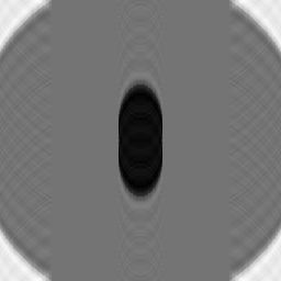
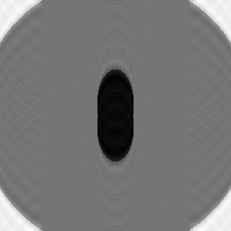
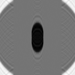
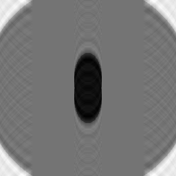
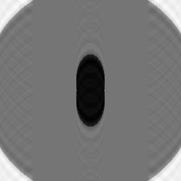
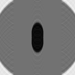
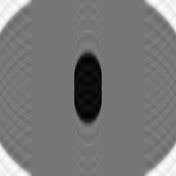
Reconstruction Gallery — 4 Scenes × 3 Scenarios
Method: CPU_baseline | Mismatch: nominal (nominal=True, perturbed=False)
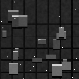
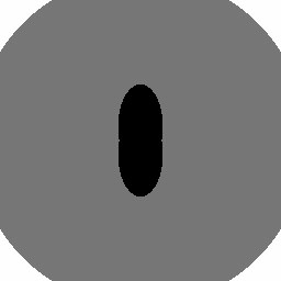
Ground Truth
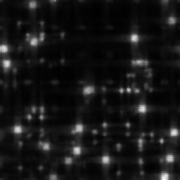
Measurement

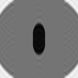
Reconstruction
Ground Truth

Measurement

Reconstruction
Ground Truth
Measurement (perturbed)

Reconstruction


Mean PSNR Across All Scenes
Per-scene PSNR breakdown (4 scenes)
| Scene | I (PSNR) | I (SSIM) | II (PSNR) | II (SSIM) | III (PSNR) | III (SSIM) |
|---|---|---|---|---|---|---|
| scene_00 | 15.503504478809369 | 0.2341635915614249 | 15.447084365158803 | 0.2373800670650224 | 15.545546774161242 | 0.23052417070261594 |
| scene_01 | 29.027661217474883 | 0.8684057272970452 | 28.58935657255064 | 0.8712144155448451 | 31.592415537777523 | 0.9075777438597679 |
| scene_02 | 29.227212879824922 | 0.8516233712949678 | 28.334155500148754 | 0.8570647803988047 | 31.36543035296549 | 0.8997771391179263 |
| scene_03 | 28.22777093634853 | 0.8776792969503701 | 29.575687028393908 | 0.8479275774293132 | 32.56408008462443 | 0.8954795385690928 |
| Mean | 25.496537378114425 | 0.707967996775952 | 25.486570866563028 | 0.7033967101094963 | 27.766868187382173 | 0.7333396480623507 |
Experimental Setup
Key References
- Cumming & Wong, 'Digital Processing of Synthetic Aperture Radar Data', Artech House (2005)
- Torres et al., 'GMES Sentinel-1 mission', Remote Sensing of Environment 120, 9-24 (2012)
Canonical Datasets
- SEN12MS (Schmitt et al., multi-modal Sentinel-1/2)
- SpaceNet 6 (SAR building footprints)
Spec DAG — Forward Model Pipeline
F(azimuth×range) → D(g, η₁)
Mismatch Parameters
| Symbol | Parameter | Description | Nominal | Perturbed |
|---|---|---|---|---|
| Δr_a | motion_error | Platform motion error (cm) | 0 | 2.0 |
| Δφ | phase_error | Autofocus phase error (rad) | 0 | 0.3 |
| ΔRCM | range_cell_migration | Range cell migration error (cells) | 0 | 0.5 |
Credits System
Spec Primitives Reference (11 primitives)
Free-space or medium propagation kernel (Fresnel, Rayleigh-Sommerfeld).
Spatial or spatio-temporal amplitude modulation (coded aperture, SLM pattern).
Geometric projection operator (Radon transform, fan-beam, cone-beam).
Sampling in the Fourier / k-space domain (MRI, ptychography).
Shift-invariant convolution with a point-spread function (PSF).
Summation along a physical dimension (spectral, temporal, angular).
Sensor readout with gain g and noise model η (Gaussian, Poisson, mixed).
Patterned illumination (block, Hadamard, random) applied to the scene.
Spectral dispersion element (prism, grating) with shift α and aperture a.
Sample or gantry rotation (CT, electron tomography).
Spectral filter or monochromator selecting a wavelength band.