Proton Radiography
Proton Radiography
Standard reconstruction benchmark — forward model perfectly known, no calibration needed. Score = 0.5 × clip((PSNR−15)/30, 0, 1) + 0.5 × SSIM
| # | Method | Score | PSNR (dB) | SSIM | Source | |
|---|---|---|---|---|---|---|
| 🥇 |
pCT-Former
pCT-Former Proton CT transformer, 2024
33.0 dB
SSIM 0.920
Checkpoint unavailable
|
0.760 | 33.0 | 0.920 | ✓ Certified | Proton CT transformer, 2024 |
| 🥈 |
ProtonNet
ProtonNet Proton CT DL, 2022
31.0 dB
SSIM 0.890
Checkpoint unavailable
|
0.712 | 31.0 | 0.890 | ✓ Certified | Proton CT DL, 2022 |
| 🥉 | DROP-TVS | 0.595 | 27.0 | 0.790 | ✓ Certified | Penfold et al., 2010 |
| 4 | FBP-MLP | 0.467 | 23.5 | 0.650 | ✓ Certified | Schulte et al., 2008 |
Dataset: PWM Benchmark (4 algorithms)
Blind Reconstruction Challenge — forward model has unknown mismatch, must calibrate from data. Score = 0.4 × PSNR_norm + 0.4 × SSIM + 0.2 × (1 − ‖y − Ĥx̂‖/‖y‖)
| # | Method | Overall Score | Public PSNR / SSIM |
Dev PSNR / SSIM |
Hidden PSNR / SSIM |
Trust | Source |
|---|---|---|---|---|---|---|---|
| 🥇 | pCT-Former + gradient | 0.710 |
0.751
30.15 dB / 0.919
|
0.709
28.05 dB / 0.882
|
0.670
27.11 dB / 0.861
|
✓ Certified | Proton CT transformer, 2024 |
| 🥈 | ProtonNet + gradient | 0.584 |
0.718
28.28 dB / 0.887
|
0.536
21.42 dB / 0.665
|
0.497
19.92 dB / 0.595
|
✓ Certified | Proton CT DL reconstruction, 2022 |
| 🥉 | DROP-TVS + gradient | 0.575 |
0.674
25.85 dB / 0.828
|
0.553
21.26 dB / 0.657
|
0.498
20.07 dB / 0.602
|
✓ Certified | Penfold et al., Med. Phys. 2010 |
| 4 | FBP-MLP + gradient | 0.537 |
0.547
20.95 dB / 0.643
|
0.534
21.15 dB / 0.652
|
0.529
20.9 dB / 0.641
|
✓ Certified | Schulte et al., Med. Phys. 2008 |
Complete score requires all 3 tiers (Public + Dev + Hidden).
Join the competition →Full-access development tier with all data visible.
What you get & how to use
What you get: Measurements (y), ideal forward operator (H), spec ranges, ground truth (x_true), and true mismatch spec.
How to use: Load HDF5 → compare reconstruction vs x_true → check consistency → iterate.
What to submit: Reconstructed signals (x_hat) and corrected spec as HDF5.
Public Leaderboard
| # | Method | Score | PSNR | SSIM |
|---|---|---|---|---|
| 1 | pCT-Former + gradient | 0.751 | 30.15 | 0.919 |
| 2 | ProtonNet + gradient | 0.718 | 28.28 | 0.887 |
| 3 | DROP-TVS + gradient | 0.674 | 25.85 | 0.828 |
| 4 | FBP-MLP + gradient | 0.547 | 20.95 | 0.643 |
Spec Ranges (3 parameters)
| Parameter | Min | Max | Unit |
|---|---|---|---|
| energy_loss | -2.0 | 4.0 | % |
| scattering | -5.0 | 10.0 | % |
| range_straggling | -3.0 | 6.0 | % |
Blind evaluation tier — no ground truth available.
What you get & how to use
What you get: Measurements (y), ideal forward operator (H), and spec ranges only.
How to use: Apply your pipeline from the Public tier. Use consistency as self-check.
What to submit: Reconstructed signals and corrected spec. Scored server-side.
Dev Leaderboard
| # | Method | Score | PSNR | SSIM |
|---|---|---|---|---|
| 1 | pCT-Former + gradient | 0.709 | 28.05 | 0.882 |
| 2 | DROP-TVS + gradient | 0.553 | 21.26 | 0.657 |
| 3 | ProtonNet + gradient | 0.536 | 21.42 | 0.665 |
| 4 | FBP-MLP + gradient | 0.534 | 21.15 | 0.652 |
Spec Ranges (3 parameters)
| Parameter | Min | Max | Unit |
|---|---|---|---|
| energy_loss | -2.4 | 3.6 | % |
| scattering | -6.0 | 9.0 | % |
| range_straggling | -3.6 | 5.4 | % |
Fully blind server-side evaluation — no data download.
What you get & how to use
What you get: No data downloadable. Algorithm runs server-side on hidden measurements.
How to use: Package algorithm as Docker container / Python script. Submit via link.
What to submit: Containerized algorithm accepting y + H, outputting x_hat + corrected spec.
Hidden Leaderboard
| # | Method | Score | PSNR | SSIM |
|---|---|---|---|---|
| 1 | pCT-Former + gradient | 0.670 | 27.11 | 0.861 |
| 2 | FBP-MLP + gradient | 0.529 | 20.9 | 0.641 |
| 3 | DROP-TVS + gradient | 0.498 | 20.07 | 0.602 |
| 4 | ProtonNet + gradient | 0.497 | 19.92 | 0.595 |
Spec Ranges (3 parameters)
| Parameter | Min | Max | Unit |
|---|---|---|---|
| energy_loss | -1.4 | 4.6 | % |
| scattering | -3.5 | 11.5 | % |
| range_straggling | -2.1 | 6.9 | % |
Blind Reconstruction Challenge
ChallengeGiven measurements with unknown mismatch and spec ranges (not exact params), reconstruct the original signal. A method must be evaluated on all three tiers for a complete score. Scored on a composite metric: 0.4 × PSNR_norm + 0.4 × SSIM + 0.2 × (1 − ‖y − Ĥx̂‖/‖y‖).
Measurements y, ideal forward model H, spec ranges
Reconstructed signal x̂
About the Imaging Modality
Proton radiography/CT uses high-energy proton beams (100-250 MeV) to image the relative stopping power (RSP) of tissue, which is the quantity directly needed for proton therapy treatment planning. Unlike X-rays which measure attenuation, proton imaging measures the energy loss and scattering of individual protons as they traverse the object. Each proton's entry/exit position and angle are tracked, and the residual energy is measured. The RSP is reconstructed from many proton histories using iterative algorithms. Challenges include multiple Coulomb scattering (which blurs the spatial resolution to ~1 mm) and the need for single-proton tracking at high rates.
Principle
Proton radiography images the transmission and scattering of high-energy protons (50-800 MeV) through dense objects. Unlike X-rays, protons undergo significant multiple Coulomb scattering (MCS) in matter, which provides density and compositional contrast. Both transmission (energy loss) and scattering angle measurements contribute to image formation. Proton radiography can penetrate very dense materials (steel, depleted uranium) that are opaque to X-rays.
How to Build the System
Requires a high-energy proton accelerator facility (synchrotron or cyclotron delivering 200-800 MeV protons). The object is placed in the beam path between tracking detectors (silicon strip or GEM detectors) that measure each proton's position and angle before and after the object. A magnetic spectrometer (quadrupole lens system, e.g., at LANL pRad facility) focuses transmitted protons onto a scintillator + camera detector.
Common Reconstruction Algorithms
- Most Likely Path (MLP) estimation for proton CT reconstruction
- Filtered back-projection with scattering-angle weighting
- Algebraic reconstruction (ART) with MCS forward model
- Material discrimination from dual-parameter (transmission + scattering) analysis
- Deep-learning proton CT reconstruction for reduced view angles
Common Mistakes
- Ignoring multiple Coulomb scattering in the reconstruction model, causing blur
- Nuclear interaction losses (protons stopped or scattered out of detector acceptance)
- Insufficient proton statistics leading to noisy images
- Energy straggling not modeled, causing depth-of-field blur in radiography
- Detector alignment errors between upstream and downstream tracking systems
How to Avoid Mistakes
- Use MLP or cubic spline path estimation in iterative reconstruction algorithms
- Account for nuclear interaction losses in the forward model; filter outlier tracks
- Accumulate sufficient proton histories (>10⁶ for radiography, >10⁸ for proton CT)
- Include energy straggling in the forward model or use higher energy protons to reduce it
- Carefully align tracking detectors with survey or use track-based alignment algorithms
Forward-Model Mismatch Cases
- The widefield fallback applies Gaussian blur, but proton radiography measures energy loss and multiple Coulomb scattering (MCS) of high-energy protons traversing the object — the scattering angle distribution encodes areal density, not spatial blur
- Protons lose energy continuously (Bethe-Bloch formula: -dE/dx ~ Z/A * z^2/beta^2) and scatter via Coulomb interaction — the measurement combines transmission intensity, residual energy, and scattering angle, none of which are modeled by optical blur
How to Correct the Mismatch
- Use the proton radiography operator that models energy-dependent proton transport: energy loss via Bethe-Bloch stopping power and angular broadening via Highland MCS formula (theta_rms ~ 13.6 MeV/(p*v) * sqrt(t/X_0))
- Reconstruct water-equivalent path length (WEPL) maps from residual energy measurements, or use scattering radiography for material discrimination — essential for proton therapy treatment planning
Experimental Setup — Signal Chain

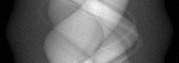
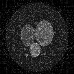
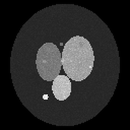
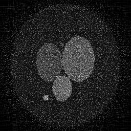
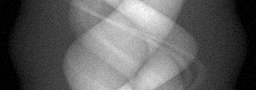
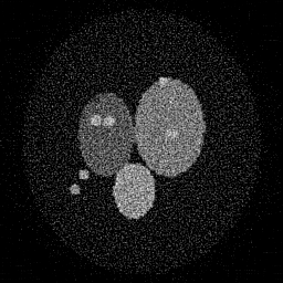
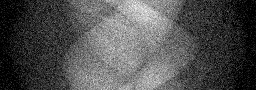
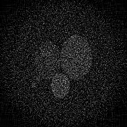
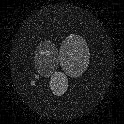
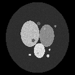
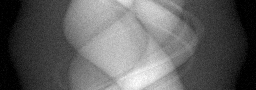
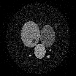
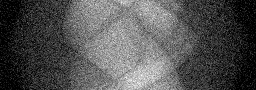
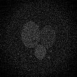
Reconstruction Gallery — 4 Scenes × 3 Scenarios
Method: CPU_baseline | Mismatch: nominal (nominal=True, perturbed=False)

Ground Truth
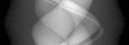
Measurement

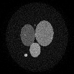
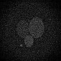
Reconstruction
Ground Truth
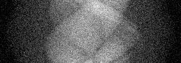
Measurement
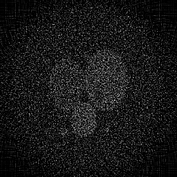
Reconstruction
Ground Truth
Measurement (perturbed)
Reconstruction


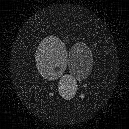
Mean PSNR Across All Scenes
Per-scene PSNR breakdown (4 scenes)
| Scene | I (PSNR) | I (SSIM) | II (PSNR) | II (SSIM) | III (PSNR) | III (SSIM) |
|---|---|---|---|---|---|---|
| scene_00 | 16.584200964385797 | 0.3250905580130585 | 12.506523882319042 | 0.044716474341606735 | 15.931719256055723 | 0.12142227244746187 |
| scene_01 | 18.884299556167566 | 0.3252411352628261 | 13.742128073130111 | 0.048029248758291385 | 17.02391116326154 | 0.11622117666622035 |
| scene_02 | 18.301830801494646 | 0.32976160086547746 | 13.36792873190369 | 0.04964364838717723 | 16.550610792224443 | 0.1259030967011571 |
| scene_03 | 16.67775192548055 | 0.3247822274360334 | 12.53195005733068 | 0.044966709218701925 | 15.850507045662987 | 0.12621817875162467 |
| Mean | 17.61202081188214 | 0.3262188803943489 | 13.037132686170882 | 0.046839020176444326 | 16.33918706430117 | 0.122441181141616 |
Experimental Setup
Key References
- Schulte et al., 'Conceptual design of a proton computed tomography system for applications in proton radiation therapy', IEEE Trans. Nucl. Sci. 51, 866-872 (2004)
Canonical Datasets
- Simulated proton CT phantoms (Penfold et al.)
Spec DAG — Forward Model Pipeline
Π(proton) → D(g, η₁)
Mismatch Parameters
| Symbol | Parameter | Description | Nominal | Perturbed |
|---|---|---|---|---|
| ΔS | energy_loss | Stopping power error (%) | 0 | 2.0 |
| Δθ_MCS | scattering | Multiple Coulomb scattering error (%) | 0 | 5.0 |
| ΔR | range_straggling | Range straggling error (%) | 0 | 3.0 |
Credits System
Spec Primitives Reference (11 primitives)
Free-space or medium propagation kernel (Fresnel, Rayleigh-Sommerfeld).
Spatial or spatio-temporal amplitude modulation (coded aperture, SLM pattern).
Geometric projection operator (Radon transform, fan-beam, cone-beam).
Sampling in the Fourier / k-space domain (MRI, ptychography).
Shift-invariant convolution with a point-spread function (PSF).
Summation along a physical dimension (spectral, temporal, angular).
Sensor readout with gain g and noise model η (Gaussian, Poisson, mixed).
Patterned illumination (block, Hadamard, random) applied to the scene.
Spectral dispersion element (prism, grating) with shift α and aperture a.
Sample or gantry rotation (CT, electron tomography).
Spectral filter or monochromator selecting a wavelength band.