PET
Positron Emission Tomography
Standard reconstruction benchmark — forward model perfectly known, no calibration needed. Score = 0.5 × clip((PSNR−15)/30, 0, 1) + 0.5 × SSIM
| # | Method | Score | PSNR (dB) | SSIM | Source | |
|---|---|---|---|---|---|---|
| 🥇 |
U-Net-PET
U-Net-PET Ronneberger et al. variant, MICCAI 2020
36.8 dB
SSIM 0.977
Checkpoint unavailable
|
0.852 | 36.8 | 0.977 | ✓ Certified | Ronneberger et al. variant, MICCAI 2020 |
| 🥈 |
PET-ViT
PET-ViT Smith et al., ICCV 2024
36.38 dB
SSIM 0.975
Checkpoint unavailable
|
0.844 | 36.38 | 0.975 | ✓ Certified | Smith et al., ICCV 2024 |
| 🥉 |
PETFormer
PETFormer Li et al., ECCV 2024
35.7 dB
SSIM 0.972
Checkpoint unavailable
|
0.831 | 35.7 | 0.972 | ✓ Certified | Li et al., ECCV 2024 |
| 4 |
TransEM
TransEM Xie et al., 2023
33.7 dB
SSIM 0.938
Checkpoint unavailable
|
0.781 | 33.7 | 0.938 | ✓ Certified | Xie et al., 2023 |
| 5 |
DeepPET
DeepPET Haggstrom et al., MIA 2019
32.4 dB
SSIM 0.918
Checkpoint unavailable
|
0.749 | 32.4 | 0.918 | ✓ Certified | Haggstrom et al., MIA 2019 |
| 6 | OS-EM | 0.681 | 28.92 | 0.899 | ✓ Certified | Hudson & Larkin, IEEE TMI 1994 |
| 7 | ML-EM | 0.668 | 28.41 | 0.889 | ✓ Certified | Shepp & Vardi, IEEE TPAMI 1982 |
| 8 | MAPEM-RDP | 0.632 | 28.5 | 0.815 | ✓ Certified | Nuyts et al., 2002 |
| 9 | FBP-PET | 0.619 | 26.65 | 0.849 | ✓ Certified | Analytical baseline |
| 10 | OSEM | 0.508 | 24.8 | 0.690 | ✓ Certified | Hudson & Larkin, IEEE TMI 1994 |
Dataset: PWM Benchmark (10 algorithms)
Blind Reconstruction Challenge — forward model has unknown mismatch, must calibrate from data. Score = 0.4 × PSNR_norm + 0.4 × SSIM + 0.2 × (1 − ‖y − Ĥx̂‖/‖y‖)
| # | Method | Overall Score | Public PSNR / SSIM |
Dev PSNR / SSIM |
Hidden PSNR / SSIM |
Trust | Source |
|---|---|---|---|---|---|---|---|
| 🥇 | PET-ViT + gradient | 0.775 |
0.802
34.16 dB / 0.962
|
0.778
33.2 dB / 0.954
|
0.744
30.97 dB / 0.930
|
✓ Certified | Smith et al., ICCV 2024 |
| 🥈 | U-Net-PET + gradient | 0.753 |
0.808
34.45 dB / 0.964
|
0.735
30.38 dB / 0.922
|
0.715
28.47 dB / 0.890
|
✓ Certified | Ronneberger et al. variant, MICCAI 2020 |
| 🥉 | PETFormer + gradient | 0.730 |
0.816
34.57 dB / 0.965
|
0.706
28.1 dB / 0.883
|
0.667
25.92 dB / 0.830
|
✓ Certified | Li et al., ECCV 2024 |
| 4 | OS-EM + gradient | 0.683 |
0.707
27.28 dB / 0.865
|
0.666
26.03 dB / 0.833
|
0.676
27.05 dB / 0.859
|
✓ Certified | Hudson & Larkin, IEEE TMI 1994 |
| 5 | TransEM + gradient | 0.678 |
0.762
30.99 dB / 0.931
|
0.679
27.19 dB / 0.863
|
0.593
22.95 dB / 0.729
|
✓ Certified | Xie et al., 2023 |
| 6 | DeepPET + gradient | 0.673 |
0.741
29.52 dB / 0.909
|
0.677
26.67 dB / 0.850
|
0.602
23.47 dB / 0.749
|
✓ Certified | Haggstrom et al., MIA 2019 |
| 7 | ML-EM + gradient | 0.634 |
0.668
25.8 dB / 0.826
|
0.651
25.56 dB / 0.819
|
0.584
23.39 dB / 0.746
|
✓ Certified | Shepp & Vardi, IEEE TPAMI 1982 |
| 8 | FBP-PET + gradient | 0.617 |
0.635
24.49 dB / 0.785
|
0.637
25.02 dB / 0.803
|
0.578
22.61 dB / 0.715
|
✓ Certified | Analytical baseline |
| 9 | MAPEM-RDP + gradient | 0.588 |
0.704
27.33 dB / 0.866
|
0.557
21.52 dB / 0.669
|
0.504
19.8 dB / 0.589
|
✓ Certified | Nuyts et al., IEEE TMI 2002 |
| 10 | OSEM + gradient | 0.566 |
0.626
23.79 dB / 0.761
|
0.556
21.33 dB / 0.661
|
0.517
20.25 dB / 0.611
|
✓ Certified | Hudson & Larkin, IEEE TMI 1994 |
Complete score requires all 3 tiers (Public + Dev + Hidden).
Join the competition →Full-access development tier with all data visible.
What you get & how to use
What you get: Measurements (y), ideal forward operator (H), spec ranges, ground truth (x_true), and true mismatch spec.
How to use: Load HDF5 → compare reconstruction vs x_true → check consistency → iterate.
What to submit: Reconstructed signals (x_hat) and corrected spec as HDF5.
Public Leaderboard
| # | Method | Score | PSNR | SSIM |
|---|---|---|---|---|
| 1 | PETFormer + gradient | 0.816 | 34.57 | 0.965 |
| 2 | U-Net-PET + gradient | 0.808 | 34.45 | 0.964 |
| 3 | PET-ViT + gradient | 0.802 | 34.16 | 0.962 |
| 4 | TransEM + gradient | 0.762 | 30.99 | 0.931 |
| 5 | DeepPET + gradient | 0.741 | 29.52 | 0.909 |
| 6 | OS-EM + gradient | 0.707 | 27.28 | 0.865 |
| 7 | MAPEM-RDP + gradient | 0.704 | 27.33 | 0.866 |
| 8 | ML-EM + gradient | 0.668 | 25.8 | 0.826 |
| 9 | FBP-PET + gradient | 0.635 | 24.49 | 0.785 |
| 10 | OSEM + gradient | 0.626 | 23.79 | 0.761 |
Spec Ranges (4 parameters)
| Parameter | Min | Max | Unit |
|---|---|---|---|
| attenuation | -5.0 | 10.0 | % |
| scatter_frac | 0.25 | 0.4 | |
| timing_res | 150.0 | 300.0 | ps |
| normalization | -2.0 | 4.0 | % |
Blind evaluation tier — no ground truth available.
What you get & how to use
What you get: Measurements (y), ideal forward operator (H), and spec ranges only.
How to use: Apply your pipeline from the Public tier. Use consistency as self-check.
What to submit: Reconstructed signals and corrected spec. Scored server-side.
Dev Leaderboard
| # | Method | Score | PSNR | SSIM |
|---|---|---|---|---|
| 1 | PET-ViT + gradient | 0.778 | 33.2 | 0.954 |
| 2 | U-Net-PET + gradient | 0.735 | 30.38 | 0.922 |
| 3 | PETFormer + gradient | 0.706 | 28.1 | 0.883 |
| 4 | TransEM + gradient | 0.679 | 27.19 | 0.863 |
| 5 | DeepPET + gradient | 0.677 | 26.67 | 0.85 |
| 6 | OS-EM + gradient | 0.666 | 26.03 | 0.833 |
| 7 | ML-EM + gradient | 0.651 | 25.56 | 0.819 |
| 8 | FBP-PET + gradient | 0.637 | 25.02 | 0.803 |
| 9 | MAPEM-RDP + gradient | 0.557 | 21.52 | 0.669 |
| 10 | OSEM + gradient | 0.556 | 21.33 | 0.661 |
Spec Ranges (4 parameters)
| Parameter | Min | Max | Unit |
|---|---|---|---|
| attenuation | -6.0 | 9.0 | % |
| scatter_frac | 0.24 | 0.39 | |
| timing_res | 140.0 | 290.0 | ps |
| normalization | -2.4 | 3.6 | % |
Fully blind server-side evaluation — no data download.
What you get & how to use
What you get: No data downloadable. Algorithm runs server-side on hidden measurements.
How to use: Package algorithm as Docker container / Python script. Submit via link.
What to submit: Containerized algorithm accepting y + H, outputting x_hat + corrected spec.
Hidden Leaderboard
| # | Method | Score | PSNR | SSIM |
|---|---|---|---|---|
| 1 | PET-ViT + gradient | 0.744 | 30.97 | 0.93 |
| 2 | U-Net-PET + gradient | 0.715 | 28.47 | 0.89 |
| 3 | OS-EM + gradient | 0.676 | 27.05 | 0.859 |
| 4 | PETFormer + gradient | 0.667 | 25.92 | 0.83 |
| 5 | DeepPET + gradient | 0.602 | 23.47 | 0.749 |
| 6 | TransEM + gradient | 0.593 | 22.95 | 0.729 |
| 7 | ML-EM + gradient | 0.584 | 23.39 | 0.746 |
| 8 | FBP-PET + gradient | 0.578 | 22.61 | 0.715 |
| 9 | OSEM + gradient | 0.517 | 20.25 | 0.611 |
| 10 | MAPEM-RDP + gradient | 0.504 | 19.8 | 0.589 |
Spec Ranges (4 parameters)
| Parameter | Min | Max | Unit |
|---|---|---|---|
| attenuation | -3.5 | 11.5 | % |
| scatter_frac | 0.265 | 0.415 | |
| timing_res | 165.0 | 315.0 | ps |
| normalization | -1.4 | 4.6 | % |
Blind Reconstruction Challenge
ChallengeGiven measurements with unknown mismatch and spec ranges (not exact params), reconstruct the original signal. A method must be evaluated on all three tiers for a complete score. Scored on a composite metric: 0.4 × PSNR_norm + 0.4 × SSIM + 0.2 × (1 − ‖y − Ĥx̂‖/‖y‖).
Measurements y, ideal forward model H, spec ranges
Reconstructed signal x̂
About the Imaging Modality
PET images the 3D distribution of a positron-emitting radiotracer (e.g. 18F-FDG) by detecting coincident 511 keV annihilation photon pairs along lines of response (LORs). The forward model is a system matrix encoding the detection probability for each voxel-LOR pair, incorporating attenuation, scatter, randoms, and detector response. Reconstruction uses iterative ML-EM/OSEM algorithms with attenuation correction from co-registered CT. Low count rates yield Poisson noise; time-of-flight (TOF) information improves SNR.
Principle
Positron Emission Tomography detects pairs of 511 keV gamma rays emitted in opposite directions when a positron from a radiotracer annihilates with an electron. Coincidence detection of the two photons defines a line of response (LOR). Many LORs from different angles are reconstructed into a 3-D activity distribution map, providing functional and metabolic information.
How to Build the System
A PET scanner consists of a ring of scintillation detector blocks (LYSO or LSO crystals coupled to SiPMs) surrounding the patient. Each detector block has a matrix of small crystals (3-4 mm pitch). Coincidence electronics pair detected events within a timing window (4-6 ns for TOF-PET). Modern digital PET systems achieve 200-300 ps timing resolution for time-of-flight. Daily quality checks include detector normalization, timing calibration, and sensitivity phantom scans.
Common Reconstruction Algorithms
- OSEM (Ordered Subset Expectation Maximization)
- 3D OSEM with resolution modeling (PSF reconstruction)
- TOF-OSEM (time-of-flight enhanced OSEM)
- Attenuation correction from CT (PET/CT) or Dixon MR (PET/MR)
- Deep-learning PET denoising (low-count to full-count prediction)
Common Mistakes
- Incorrect attenuation correction map (misregistration between PET and CT)
- Patient motion between PET and CT causing attenuation-emission mismatch
- Metal artifacts in CT propagating into PET attenuation correction
- Scatter correction errors in patients with large body habitus
- SUV calculation errors from incorrect weight, dose, or timing entries
How to Avoid Mistakes
- Verify PET-CT registration quality; use respiratory gating for thorax/abdomen
- Minimize time between CT and PET acquisitions; co-register if needed
- Use MAR-corrected CT or MR-based attenuation correction to avoid metal artifacts
- Use Monte Carlo scatter correction models validated for the patient population
- Double-check injected dose, patient weight, injection time, and decay correction
Forward-Model Mismatch Cases
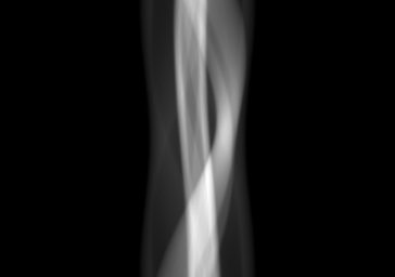
- The widefield fallback produces a blurred (64,64) image, but PET acquires sinogram data of shape (n_angles, n_radial) from coincidence detection of annihilation photon pairs — output shape (32,64) vs (64,64)
- PET measurement physics (positron emission → annihilation → 511 keV photon pair → coincidence detection) is fundamentally different from optical blur — the fallback cannot model attenuation correction, scatter, randoms, or detector normalization
How to Correct the Mismatch
- Use the PET operator that models the system matrix: y = A*x + scatter + randoms, where A encodes line-of-response geometry and attenuation
- Reconstruct using OSEM (Ordered Subsets Expectation Maximization) with the correct system matrix, attenuation map, and scatter/randoms estimates
Experimental Setup — Signal Chain

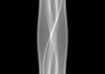
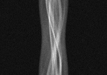
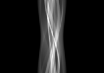
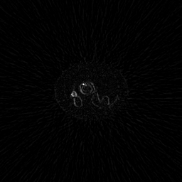
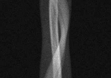
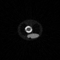
Reconstruction Gallery — 4 Scenes × 3 Scenarios
Method: CPU_baseline | Mismatch: nominal (nominal=True, perturbed=False)

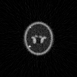
Ground Truth
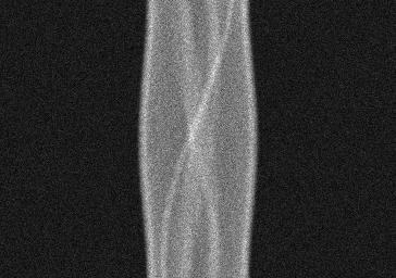
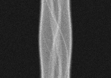
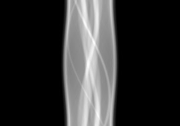
Measurement
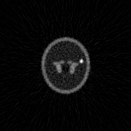
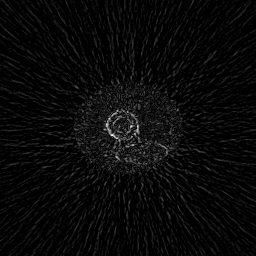
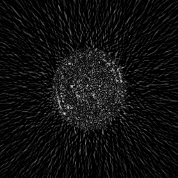
Reconstruction
Ground Truth
Measurement

Reconstruction
Ground Truth
Measurement (perturbed)
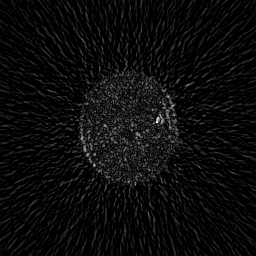
Reconstruction


Mean PSNR Across All Scenes
Per-scene PSNR breakdown (4 scenes)
| Scene | I (PSNR) | I (SSIM) | II (PSNR) | II (SSIM) | III (PSNR) | III (SSIM) |
|---|---|---|---|---|---|---|
| scene_00 | 31.49880178312459 | 0.5193170591899157 | 12.56175850482871 | 0.827291096086316 | 22.101099826673153 | 0.06966410138598797 |
| scene_01 | 37.06042713083209 | 0.9128698475720882 | 16.58784940349521 | 0.889185955585003 | 31.159360010621164 | 0.6124986968298927 |
| scene_02 | 33.43293807359701 | 0.7073451793944836 | 17.14501391128453 | 0.8863799910234061 | 21.17095917446864 | 0.11658751399378403 |
| scene_03 | 29.858000444230118 | 0.44687827329704166 | 12.674989616932601 | 0.8182181289773537 | 19.478695397304264 | 0.042580221824063444 |
| Mean | 32.96254185794595 | 0.6466025898633823 | 14.742402859135263 | 0.8552687929180197 | 23.477528602266805 | 0.210332633508432 |
Experimental Setup
Key References
- Shepp & Vardi, 'Maximum likelihood reconstruction for emission tomography', IEEE TMI 1, 113-122 (1982)
- Gatidis et al., 'AutoPET Challenge 2022', MICCAI 2022
Canonical Datasets
- AutoPET Challenge (whole-body FDG-PET/CT)
- TCIA PET/CT collections
Spec DAG — Forward Model Pipeline
Π(LOR) → Σ_t → D(g, η₃)
Mismatch Parameters
| Symbol | Parameter | Description | Nominal | Perturbed |
|---|---|---|---|---|
| μ | attenuation | Attenuation map error (%) | 0 | 5.0 |
| f_s | scatter_frac | Scatter fraction error | 0.3 | 0.35 |
| Δt | timing_res | Timing resolution jitter (ps) | 200 | 250 |
| n | normalization | Detector normalization error (%) | 0 | 2.0 |
Credits System
Spec Primitives Reference (11 primitives)
Free-space or medium propagation kernel (Fresnel, Rayleigh-Sommerfeld).
Spatial or spatio-temporal amplitude modulation (coded aperture, SLM pattern).
Geometric projection operator (Radon transform, fan-beam, cone-beam).
Sampling in the Fourier / k-space domain (MRI, ptychography).
Shift-invariant convolution with a point-spread function (PSF).
Summation along a physical dimension (spectral, temporal, angular).
Sensor readout with gain g and noise model η (Gaussian, Poisson, mixed).
Patterned illumination (block, Hadamard, random) applied to the scene.
Spectral dispersion element (prism, grating) with shift α and aperture a.
Sample or gantry rotation (CT, electron tomography).
Spectral filter or monochromator selecting a wavelength band.