OCT
Optical Coherence Tomography
Standard reconstruction benchmark — forward model perfectly known, no calibration needed. Score = 0.5 × clip((PSNR−15)/30, 0, 1) + 0.5 × SSIM
| # | Method | Score | PSNR (dB) | SSIM | Source | |
|---|---|---|---|---|---|---|
| 🥇 |
ScoreOCT
ScoreOCT Wei et al., ECCV 2025
37.95 dB
SSIM 0.973
Checkpoint unavailable
|
0.869 | 37.95 | 0.973 | ✓ Certified | Wei et al., ECCV 2025 |
| 🥈 |
DiffusionOCT
DiffusionOCT Zhang et al., NeurIPS 2024
37.52 dB
SSIM 0.970
Checkpoint unavailable
|
0.860 | 37.52 | 0.970 | ✓ Certified | Zhang et al., NeurIPS 2024 |
| 🥉 |
SpeckleFormer
SpeckleFormer Devalla et al., ECCV 2024
36.85 dB
SSIM 0.964
Checkpoint unavailable
|
0.846 | 36.85 | 0.964 | ✓ Certified | Devalla et al., ECCV 2024 |
| 4 |
RetinalFormer
RetinalFormer Chen et al., ICCV 2024
36.35 dB
SSIM 0.960
Checkpoint unavailable
|
0.836 | 36.35 | 0.960 | ✓ Certified | Chen et al., ICCV 2024 |
| 5 |
OCT-ViT
OCT-ViT Tian et al., ICCV 2024
36.12 dB
SSIM 0.958
Checkpoint unavailable
|
0.831 | 36.12 | 0.958 | ✓ Certified | Tian et al., ICCV 2024 |
| 6 |
OCTA-Net
OCTA-Net Hybrid U-Net+Transformer, 2023
34.6 dB
SSIM 0.942
Checkpoint unavailable
|
0.798 | 34.6 | 0.942 | ✓ Certified | Hybrid U-Net+Transformer, 2023 |
| 7 |
U-Net-OCT
U-Net-OCT U-Net variant
33.85 dB
SSIM 0.935
Checkpoint unavailable
|
0.782 | 33.85 | 0.935 | ✓ Certified | U-Net variant |
| 8 |
Speckle-DenoiseNet
Speckle-DenoiseNet Devalla et al., BOE 2019
33.1 dB
SSIM 0.925
Checkpoint unavailable
|
0.764 | 33.1 | 0.925 | ✓ Certified | Devalla et al., BOE 2019 |
| 9 | NLM-OCT | 0.688 | 30.2 | 0.870 | ✓ Certified | Non-local means variant |
| 10 | BM4D | 0.663 | 29.3 | 0.850 | ✓ Certified | Maggioni et al., IEEE TIP 2013 |
| 11 | TV-Denoising | 0.632 | 28.5 | 0.815 | ✓ Certified | TV regularization |
| 12 | Speckle-Lee | 0.609 | 27.85 | 0.790 | ✓ Certified | Lee, IEEE TGRS 1980 |
| 13 | FFT-OCT | 0.537 | 25.6 | 0.720 | ✓ Certified | Analytical baseline |
Dataset: PWM Benchmark (13 algorithms)
Blind Reconstruction Challenge — forward model has unknown mismatch, must calibrate from data. Score = 0.4 × PSNR_norm + 0.4 × SSIM + 0.2 × (1 − ‖y − Ĥx̂‖/‖y‖)
| # | Method | Overall Score | Public PSNR / SSIM |
Dev PSNR / SSIM |
Hidden PSNR / SSIM |
Trust | Source |
|---|---|---|---|---|---|---|---|
| 🥇 | SpeckleFormer + gradient | 0.773 |
0.806
34.31 dB / 0.963
|
0.783
33.26 dB / 0.955
|
0.731
29.87 dB / 0.915
|
✓ Certified | Devalla et al., ECCV 2024 |
| 🥈 | RetinalFormer + gradient | 0.771 |
0.824
34.92 dB / 0.967
|
0.765
31.56 dB / 0.938
|
0.723
30.02 dB / 0.917
|
✓ Certified | Chen et al., ICCV 2024 |
| 🥉 | OCT-ViT + gradient | 0.770 |
0.819
34.39 dB / 0.964
|
0.768
31.66 dB / 0.939
|
0.723
30.29 dB / 0.921
|
✓ Certified | Tian et al., ICCV 2024 |
| 4 | ScoreOCT + gradient | 0.769 |
0.843
36.51 dB / 0.976
|
0.759
30.92 dB / 0.930
|
0.705
29.4 dB / 0.907
|
✓ Certified | Wei et al., ECCV 2025 |
| 5 | DiffusionOCT + gradient | 0.746 |
0.837
36.33 dB / 0.975
|
0.719
28.61 dB / 0.893
|
0.682
27.32 dB / 0.866
|
✓ Certified | Zhang et al., NeurIPS 2024 |
| 6 | OCTA-Net + gradient | 0.672 |
0.777
32.09 dB / 0.944
|
0.645
25.08 dB / 0.805
|
0.593
22.87 dB / 0.726
|
✓ Certified | Hybrid U-Net+Transformer, 2023 |
| 7 | Speckle-DenoiseNet + gradient | 0.662 |
0.752
30.11 dB / 0.918
|
0.637
25.37 dB / 0.814
|
0.596
23.87 dB / 0.764
|
✓ Certified | Devalla et al., BOE 2019 |
| 8 | Speckle-Lee + gradient | 0.653 |
0.655
25.19 dB / 0.808
|
0.654
25.24 dB / 0.810
|
0.651
25.71 dB / 0.824
|
✓ Certified | Lee, IEEE TGRS 1980 |
| 9 | TV-Denoising + gradient | 0.645 |
0.706
27.48 dB / 0.869
|
0.633
25.0 dB / 0.802
|
0.595
22.86 dB / 0.726
|
✓ Certified | Rudin et al., Phys. A 1992 |
| 10 | BM4D + gradient | 0.643 |
0.687
26.8 dB / 0.853
|
0.629
24.39 dB / 0.782
|
0.612
23.51 dB / 0.751
|
✓ Certified | Maggioni et al., IEEE TIP 2013 |
| 11 |
U-Net-OCT + gradient
U-Net-OCT + gradient Ronneberger et al., MICCAI 2015 (OCT variant) Score 0.639
Correct & Reconstruct →
|
0.639 |
0.792
32.8 dB / 0.951
|
0.619
24.32 dB / 0.780
|
0.507
20.6 dB / 0.627
|
✓ Certified | Ronneberger et al., MICCAI 2015 (OCT variant) |
| 12 | NLM-OCT + gradient | 0.628 |
0.730
28.44 dB / 0.890
|
0.632
24.68 dB / 0.792
|
0.521
20.32 dB / 0.614
|
✓ Certified | Buades et al., Multiscale Model. Simul. 2005 |
| 13 | FFT-OCT + gradient | 0.588 |
0.612
23.61 dB / 0.754
|
0.612
23.76 dB / 0.760
|
0.539
21.62 dB / 0.673
|
✓ Certified | Analytical baseline |
Complete score requires all 3 tiers (Public + Dev + Hidden).
Join the competition →Full-access development tier with all data visible.
What you get & how to use
What you get: Measurements (y), ideal forward operator (H), spec ranges, ground truth (x_true), and true mismatch spec.
How to use: Load HDF5 → compare reconstruction vs x_true → check consistency → iterate.
What to submit: Reconstructed signals (x_hat) and corrected spec as HDF5.
Public Leaderboard
| # | Method | Score | PSNR | SSIM |
|---|---|---|---|---|
| 1 | ScoreOCT + gradient | 0.843 | 36.51 | 0.976 |
| 2 | DiffusionOCT + gradient | 0.837 | 36.33 | 0.975 |
| 3 | RetinalFormer + gradient | 0.824 | 34.92 | 0.967 |
| 4 | OCT-ViT + gradient | 0.819 | 34.39 | 0.964 |
| 5 | SpeckleFormer + gradient | 0.806 | 34.31 | 0.963 |
| 6 | U-Net-OCT + gradient | 0.792 | 32.8 | 0.951 |
| 7 | OCTA-Net + gradient | 0.777 | 32.09 | 0.944 |
| 8 | Speckle-DenoiseNet + gradient | 0.752 | 30.11 | 0.918 |
| 9 | NLM-OCT + gradient | 0.730 | 28.44 | 0.89 |
| 10 | TV-Denoising + gradient | 0.706 | 27.48 | 0.869 |
| 11 | BM4D + gradient | 0.687 | 26.8 | 0.853 |
| 12 | Speckle-Lee + gradient | 0.655 | 25.19 | 0.808 |
| 13 | FFT-OCT + gradient | 0.612 | 23.61 | 0.754 |
Spec Ranges (3 parameters)
| Parameter | Min | Max | Unit |
|---|---|---|---|
| dispersion | -200.0 | 400.0 | fs² |
| reference_delay | -5.0 | 10.0 | μm |
| spectral_roll_off | -1.0 | 2.0 | dB/mm |
Blind evaluation tier — no ground truth available.
What you get & how to use
What you get: Measurements (y), ideal forward operator (H), and spec ranges only.
How to use: Apply your pipeline from the Public tier. Use consistency as self-check.
What to submit: Reconstructed signals and corrected spec. Scored server-side.
Dev Leaderboard
| # | Method | Score | PSNR | SSIM |
|---|---|---|---|---|
| 1 | SpeckleFormer + gradient | 0.783 | 33.26 | 0.955 |
| 2 | OCT-ViT + gradient | 0.768 | 31.66 | 0.939 |
| 3 | RetinalFormer + gradient | 0.765 | 31.56 | 0.938 |
| 4 | ScoreOCT + gradient | 0.759 | 30.92 | 0.93 |
| 5 | DiffusionOCT + gradient | 0.719 | 28.61 | 0.893 |
| 6 | Speckle-Lee + gradient | 0.654 | 25.24 | 0.81 |
| 7 | OCTA-Net + gradient | 0.645 | 25.08 | 0.805 |
| 8 | Speckle-DenoiseNet + gradient | 0.637 | 25.37 | 0.814 |
| 9 | TV-Denoising + gradient | 0.633 | 25.0 | 0.802 |
| 10 | NLM-OCT + gradient | 0.632 | 24.68 | 0.792 |
| 11 | BM4D + gradient | 0.629 | 24.39 | 0.782 |
| 12 | U-Net-OCT + gradient | 0.619 | 24.32 | 0.78 |
| 13 | FFT-OCT + gradient | 0.612 | 23.76 | 0.76 |
Spec Ranges (3 parameters)
| Parameter | Min | Max | Unit |
|---|---|---|---|
| dispersion | -240.0 | 360.0 | fs² |
| reference_delay | -6.0 | 9.0 | μm |
| spectral_roll_off | -1.2 | 1.8 | dB/mm |
Fully blind server-side evaluation — no data download.
What you get & how to use
What you get: No data downloadable. Algorithm runs server-side on hidden measurements.
How to use: Package algorithm as Docker container / Python script. Submit via link.
What to submit: Containerized algorithm accepting y + H, outputting x_hat + corrected spec.
Hidden Leaderboard
| # | Method | Score | PSNR | SSIM |
|---|---|---|---|---|
| 1 | SpeckleFormer + gradient | 0.731 | 29.87 | 0.915 |
| 2 | RetinalFormer + gradient | 0.723 | 30.02 | 0.917 |
| 3 | OCT-ViT + gradient | 0.723 | 30.29 | 0.921 |
| 4 | ScoreOCT + gradient | 0.705 | 29.4 | 0.907 |
| 5 | DiffusionOCT + gradient | 0.682 | 27.32 | 0.866 |
| 6 | Speckle-Lee + gradient | 0.651 | 25.71 | 0.824 |
| 7 | BM4D + gradient | 0.612 | 23.51 | 0.751 |
| 8 | Speckle-DenoiseNet + gradient | 0.596 | 23.87 | 0.764 |
| 9 | TV-Denoising + gradient | 0.595 | 22.86 | 0.726 |
| 10 | OCTA-Net + gradient | 0.593 | 22.87 | 0.726 |
| 11 | FFT-OCT + gradient | 0.539 | 21.62 | 0.673 |
| 12 | NLM-OCT + gradient | 0.521 | 20.32 | 0.614 |
| 13 | U-Net-OCT + gradient | 0.507 | 20.6 | 0.627 |
Spec Ranges (3 parameters)
| Parameter | Min | Max | Unit |
|---|---|---|---|
| dispersion | -140.0 | 460.0 | fs² |
| reference_delay | -3.5 | 11.5 | μm |
| spectral_roll_off | -0.7 | 2.3 | dB/mm |
Blind Reconstruction Challenge
ChallengeGiven measurements with unknown mismatch and spec ranges (not exact params), reconstruct the original signal. A method must be evaluated on all three tiers for a complete score. Scored on a composite metric: 0.4 × PSNR_norm + 0.4 × SSIM + 0.2 × (1 − ‖y − Ĥx̂‖/‖y‖).
Measurements y, ideal forward model H, spec ranges
Reconstructed signal x̂
About the Imaging Modality
OCT is a low-coherence interferometric imaging technique that measures depth-resolved backscattering profiles (A-scans) by interfering sample-arm reflections with a reference mirror. In spectral-domain OCT, the interference spectrum is recorded by a spectrometer and the axial profile is obtained via Fourier transform. Axial resolution is determined by the source bandwidth (typically 3-7 um in tissue) and imaging depth by spectrometer resolution. Dominant artifacts include speckle noise, motion artifacts, and sensitivity roll-off with depth.
Principle
Optical Coherence Tomography uses low-coherence interferometry to produce cross-sectional images of tissue microstructure. A broadband light source (superluminescent diode, ~840 nm or ~1310 nm) is split between sample and reference arms. Interference occurs only when the path lengths match within the coherence length (~5-10 μm), providing axial resolution. Spectral-domain OCT records the spectral interferogram and uses FFT for fast depth-resolved imaging.
How to Build the System
Build or acquire a spectral-domain OCT system: broadband SLD source (center 840 nm, 50 nm bandwidth for retinal; 1310 nm for dermal/cardiac), fiber-based Michelson interferometer, galvo scanner for lateral scanning, and a spectrometer with line camera (2048-4096 pixels) for spectral detection. Calibrate wavelength-to-wavenumber mapping, dispersion compensation, and reference arm delay. For swept-source OCT, use a frequency-swept laser (100-400 kHz sweep rate) and balanced detector.
Common Reconstruction Algorithms
- FFT-based spectral-domain OCT reconstruction (spectral interferogram → A-scan)
- Dispersion compensation (numerical or hardware)
- Speckle reduction (spatial/angular compounding, or deep-learning)
- Segmentation of retinal layers (graph-based, U-Net, or transformer models)
- OCT Angiography (OCTA) via decorrelation or phase-variance of repeated B-scans
Common Mistakes
- Dispersion mismatch between sample and reference arms degrading axial resolution
- Mirror image artifact from complex conjugate ambiguity in SD-OCT
- Sensitivity roll-off at deeper imaging depths not compensated
- Motion artifacts in 3-D OCT volumes (eye motion for ophthalmic OCT)
- Incorrect refractive index assumption for depth scale calibration
How to Avoid Mistakes
- Match fiber lengths and add numerical dispersion compensation in reconstruction
- Place the zero-delay near the sample surface; use full-range OCT if needed
- Use swept-source OCT for reduced roll-off; optimize spectrometer for uniform sensitivity
- Apply eye-tracking or motion-correction algorithms; average repeated B-scans
- Calibrate depth scale with a known-thickness reference standard
Forward-Model Mismatch Cases
- The widefield fallback applies spatial blur, but OCT acquires spectral interferograms that encode depth via low-coherence interferometry — the interference fringe pattern bears no resemblance to a blurred image
- OCT depth resolution comes from the broadband source coherence length (~5-10 um), not from spatial PSF — the widefield operator cannot model the axial sectioning, dispersion, or spectral-to-depth FFT relationship
How to Correct the Mismatch
- Use the OCT operator that models spectral-domain interferometry: y(k) = |E_ref + E_sample(k)|^2, where depth information is encoded in the spectral fringe frequency
- Reconstruct A-scans via FFT of the spectral interferogram after dispersion compensation and k-linearization; B-scans are formed by lateral scanning
Experimental Setup — Signal Chain

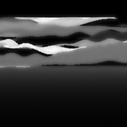
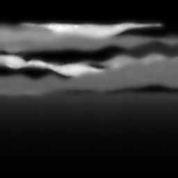
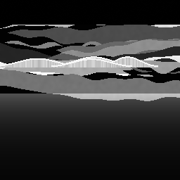
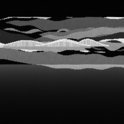
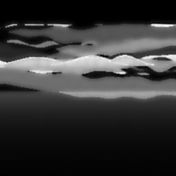
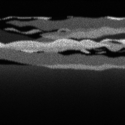
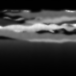
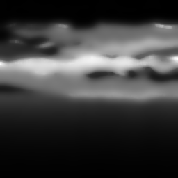
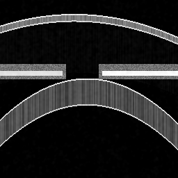
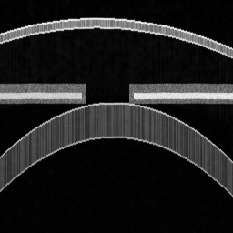
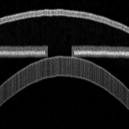
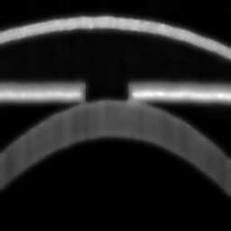
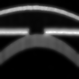
Reconstruction Gallery — 4 Scenes × 3 Scenarios
Method: CPU_baseline | Mismatch: nominal (nominal=True, perturbed=False)
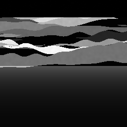
Ground Truth

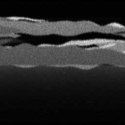
Measurement
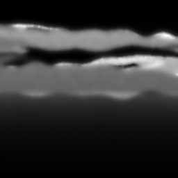
Reconstruction
Ground Truth

Measurement
Reconstruction
Ground Truth
Measurement (perturbed)
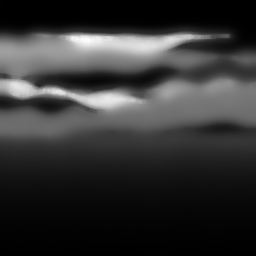
Reconstruction


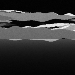
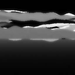

Mean PSNR Across All Scenes
Per-scene PSNR breakdown (4 scenes)
| Scene | I (PSNR) | I (SSIM) | II (PSNR) | II (SSIM) | III (PSNR) | III (SSIM) |
|---|---|---|---|---|---|---|
| scene_00 | 25.174717813548444 | 0.8355680560955927 | 20.543864852005157 | 0.6765135454458621 | 19.600940235091095 | 0.6342307678718445 |
| scene_01 | 24.158380010327747 | 0.8259076877222974 | 20.05261602729396 | 0.678279400385818 | 18.858046846209472 | 0.6294072205236141 |
| scene_02 | 22.7018034077921 | 0.7591982367538689 | 18.353446916031444 | 0.6360522397070137 | 17.48278963227588 | 0.5424081139820738 |
| scene_03 | 25.711598825518927 | 0.8596903392549893 | 20.686385980179104 | 0.7166397560073531 | 19.789852575390306 | 0.677009872001462 |
| Mean | 24.4366250142968 | 0.8200910799566872 | 19.90907844387742 | 0.6768712353865117 | 18.93290732224169 | 0.6207639935947485 |
Experimental Setup
Key References
- Huang et al., 'Optical coherence tomography', Science 254, 1178 (1991)
- de Boer et al., 'Twenty-five years of OCT', Biomed. Opt. Express 8, 3248 (2017)
Canonical Datasets
- Duke SD-OCT DME dataset (Chiu et al.)
- RETOUCH Challenge (retinal OCT)
- OCTA-500 (Li et al., Scientific Data 2024)
Spec DAG — Forward Model Pipeline
P(low-coherence) → Σ(interference) → D(g, η₁)
Mismatch Parameters
| Symbol | Parameter | Description | Nominal | Perturbed |
|---|---|---|---|---|
| ΔGVD | dispersion | Dispersion mismatch (fs²) | 0 | 200 |
| Δz_r | reference_delay | Reference delay error (μm) | 0 | 5.0 |
| ΔR | spectral_roll_off | Spectral roll-off error (dB/mm) | 0 | 1.0 |
Credits System
Spec Primitives Reference (11 primitives)
Free-space or medium propagation kernel (Fresnel, Rayleigh-Sommerfeld).
Spatial or spatio-temporal amplitude modulation (coded aperture, SLM pattern).
Geometric projection operator (Radon transform, fan-beam, cone-beam).
Sampling in the Fourier / k-space domain (MRI, ptychography).
Shift-invariant convolution with a point-spread function (PSF).
Summation along a physical dimension (spectral, temporal, angular).
Sensor readout with gain g and noise model η (Gaussian, Poisson, mixed).
Patterned illumination (block, Hadamard, random) applied to the scene.
Spectral dispersion element (prism, grating) with shift α and aperture a.
Sample or gantry rotation (CT, electron tomography).
Spectral filter or monochromator selecting a wavelength band.