Holography
Digital Holographic Microscopy
Standard reconstruction benchmark — forward model perfectly known, no calibration needed. Score = 0.5 × clip((PSNR−15)/30, 0, 1) + 0.5 × SSIM
| # | Method | Score | PSNR (dB) | SSIM | Source | |
|---|---|---|---|---|---|---|
| 🥇 |
ScorePhase
ScorePhase Wei et al., ECCV 2025
35.82 dB
SSIM 0.968
Checkpoint unavailable
|
0.831 | 35.82 | 0.968 | ✓ Certified | Wei et al., ECCV 2025 |
| 🥈 |
DiffusionPhase
DiffusionPhase Song et al., NeurIPS 2024
35.48 dB
SSIM 0.964
Checkpoint unavailable
|
0.823 | 35.48 | 0.964 | ✓ Certified | Song et al., NeurIPS 2024 |
| 🥉 |
HolographyViT
HolographyViT Wang et al., ICCV 2024
35.18 dB
SSIM 0.960
Checkpoint unavailable
|
0.816 | 35.18 | 0.960 | ✓ Certified | Wang et al., ICCV 2024 |
| 4 |
AutoPhase++
AutoPhase++ Rivenson et al., ECCV 2024
34.92 dB
SSIM 0.958
Checkpoint unavailable
|
0.811 | 34.92 | 0.958 | ✓ Certified | Rivenson et al., ECCV 2024 |
| 5 |
PhaseFormer
PhaseFormer Tian et al., ICCV 2024
34.5 dB
SSIM 0.952
Checkpoint unavailable
|
0.801 | 34.5 | 0.952 | ✓ Certified | Tian et al., ICCV 2024 |
| 6 |
PhaseResNet
PhaseResNet Baoqing et al., Optica 2023
33.15 dB
SSIM 0.942
Checkpoint unavailable
|
0.773 | 33.15 | 0.942 | ✓ Certified | Baoqing et al., Optica 2023 |
| 7 |
LRGS
LRGS Choi et al., 2023
32.8 dB
SSIM 0.935
Checkpoint unavailable
|
0.764 | 32.8 | 0.935 | ✓ Certified | Choi et al., 2023 |
| 8 |
CyclePhase
CyclePhase Ge et al., IEEE Photonics 2023
32.5 dB
SSIM 0.938
Checkpoint unavailable
|
0.761 | 32.5 | 0.938 | ✓ Certified | Ge et al., IEEE Photonics 2023 |
| 9 |
PhaseNet
PhaseNet Rivenson et al., LSA 2018
31.2 dB
SSIM 0.910
Checkpoint unavailable
|
0.725 | 31.2 | 0.910 | ✓ Certified | Rivenson et al., LSA 2018 |
| 10 |
prDeep
prDeep Metzler et al., ICML 2018
27.45 dB
SSIM 0.820
Checkpoint unavailable
|
0.617 | 27.45 | 0.820 | ✓ Certified | Metzler et al., ICML 2018 |
| 11 |
deep-PR
deep-PR Asif et al., ICCP 2017
27.2 dB
SSIM 0.810
Checkpoint unavailable
|
0.608 | 27.2 | 0.810 | ✓ Certified | Asif et al., ICCP 2017 |
| 12 | GS/HIO | 0.470 | 23.7 | 0.650 | ✓ Certified | Fienup, Appl. Opt. 1982 |
| 13 | Error Reduction | 0.438 | 22.85 | 0.615 | ✓ Certified | Fienup, J. Opt. Soc. Am. 1982 |
| 14 | Gerchberg-Saxton | 0.398 | 21.5 | 0.580 | ✓ Certified | Gerchberg & Saxton, 1972 |
Dataset: PWM Benchmark (14 algorithms)
Blind Reconstruction Challenge — forward model has unknown mismatch, must calibrate from data. Score = 0.4 × PSNR_norm + 0.4 × SSIM + 0.2 × (1 − ‖y − Ĥx̂‖/‖y‖)
| # | Method | Overall Score | Public PSNR / SSIM |
Dev PSNR / SSIM |
Hidden PSNR / SSIM |
Trust | Source |
|---|---|---|---|---|---|---|---|
| 🥇 | AutoPhase++ + gradient | 0.714 |
0.784
33.06 dB / 0.953
|
0.713
28.23 dB / 0.886
|
0.646
25.88 dB / 0.829
|
✓ Certified | Rivenson et al., ECCV 2024 |
| 🥈 | HolographyViT + gradient | 0.714 |
0.785
32.7 dB / 0.950
|
0.712
28.44 dB / 0.890
|
0.644
25.86 dB / 0.828
|
✓ Certified | Wang et al., ICCV 2024 |
| 🥉 | ScorePhase + gradient | 0.713 |
0.794
33.52 dB / 0.957
|
0.682
27.56 dB / 0.871
|
0.662
25.67 dB / 0.823
|
✓ Certified | Wei et al., ECCV 2025 |
| 4 | DiffusionPhase + gradient | 0.691 |
0.812
34.16 dB / 0.962
|
0.642
24.96 dB / 0.801
|
0.620
24.52 dB / 0.787
|
✓ Certified | Song et al., NeurIPS 2024 |
| 5 | PhaseFormer + gradient | 0.688 |
0.777
32.29 dB / 0.946
|
0.692
27.12 dB / 0.861
|
0.596
22.97 dB / 0.730
|
✓ Certified | Tian et al., ICCV 2024 |
| 6 | CyclePhase + gradient | 0.671 |
0.743
29.65 dB / 0.911
|
0.670
26.43 dB / 0.844
|
0.599
23.11 dB / 0.735
|
✓ Certified | Ge et al., IEEE Photonics 2023 |
| 7 | PhaseResNet + gradient | 0.666 |
0.780
31.48 dB / 0.937
|
0.655
25.73 dB / 0.824
|
0.562
21.87 dB / 0.684
|
✓ Certified | Baoqing et al., Optica 2023 |
| 8 | LRGS + gradient | 0.617 |
0.778
31.78 dB / 0.940
|
0.596
22.74 dB / 0.721
|
0.478
19.68 dB / 0.583
|
✓ Certified | Choi et al., 2023 |
| 9 | PhaseNet + gradient | 0.610 |
0.728
29.1 dB / 0.902
|
0.587
22.62 dB / 0.716
|
0.515
20.96 dB / 0.644
|
✓ Certified | Rivenson et al., LSA 2018 |
| 10 | prDeep + gradient | 0.550 |
0.653
25.27 dB / 0.811
|
0.537
21.23 dB / 0.656
|
0.459
18.23 dB / 0.511
|
✓ Certified | Metzler et al., ICML 2018 |
| 11 | GS/HIO + gradient | 0.518 |
0.546
20.84 dB / 0.638
|
0.534
20.58 dB / 0.626
|
0.474
18.87 dB / 0.543
|
✓ Certified | Fienup, Appl. Opt. 1982 |
| 12 | deep-PR + gradient | 0.518 |
0.652
25.43 dB / 0.815
|
0.502
19.73 dB / 0.586
|
0.401
16.69 dB / 0.435
|
✓ Certified | Asif et al., ICCP 2017 |
| 13 | Error Reduction + gradient | 0.486 |
0.574
21.76 dB / 0.680
|
0.481
18.69 dB / 0.534
|
0.404
16.59 dB / 0.430
|
✓ Certified | Fienup, J. Opt. Soc. Am. 1982 |
| 14 | Gerchberg-Saxton + gradient | 0.477 |
0.488
18.94 dB / 0.547
|
0.495
19.63 dB / 0.581
|
0.448
17.85 dB / 0.493
|
✓ Certified | Gerchberg & Saxton, Optik 1972 |
Complete score requires all 3 tiers (Public + Dev + Hidden).
Join the competition →Full-access development tier with all data visible.
What you get & how to use
What you get: Measurements (y), ideal forward operator (H), spec ranges, ground truth (x_true), and true mismatch spec.
How to use: Load HDF5 → compare reconstruction vs x_true → check consistency → iterate.
What to submit: Reconstructed signals (x_hat) and corrected spec as HDF5.
Public Leaderboard
| # | Method | Score | PSNR | SSIM |
|---|---|---|---|---|
| 1 | DiffusionPhase + gradient | 0.812 | 34.16 | 0.962 |
| 2 | ScorePhase + gradient | 0.794 | 33.52 | 0.957 |
| 3 | HolographyViT + gradient | 0.785 | 32.7 | 0.95 |
| 4 | AutoPhase++ + gradient | 0.784 | 33.06 | 0.953 |
| 5 | PhaseResNet + gradient | 0.780 | 31.48 | 0.937 |
| 6 | LRGS + gradient | 0.778 | 31.78 | 0.94 |
| 7 | PhaseFormer + gradient | 0.777 | 32.29 | 0.946 |
| 8 | CyclePhase + gradient | 0.743 | 29.65 | 0.911 |
| 9 | PhaseNet + gradient | 0.728 | 29.1 | 0.902 |
| 10 | prDeep + gradient | 0.653 | 25.27 | 0.811 |
| 11 | deep-PR + gradient | 0.652 | 25.43 | 0.815 |
| 12 | Error Reduction + gradient | 0.574 | 21.76 | 0.68 |
| 13 | GS/HIO + gradient | 0.546 | 20.84 | 0.638 |
| 14 | Gerchberg-Saxton + gradient | 0.488 | 18.94 | 0.547 |
Spec Ranges (3 parameters)
| Parameter | Min | Max | Unit |
|---|---|---|---|
| wavelength | -0.5 | 1.0 | nm |
| prop_distance | -5.0 | 10.0 | μm |
| tilt | -0.5 | 1.0 | mrad |
Blind evaluation tier — no ground truth available.
What you get & how to use
What you get: Measurements (y), ideal forward operator (H), and spec ranges only.
How to use: Apply your pipeline from the Public tier. Use consistency as self-check.
What to submit: Reconstructed signals and corrected spec. Scored server-side.
Dev Leaderboard
| # | Method | Score | PSNR | SSIM |
|---|---|---|---|---|
| 1 | AutoPhase++ + gradient | 0.713 | 28.23 | 0.886 |
| 2 | HolographyViT + gradient | 0.712 | 28.44 | 0.89 |
| 3 | PhaseFormer + gradient | 0.692 | 27.12 | 0.861 |
| 4 | ScorePhase + gradient | 0.682 | 27.56 | 0.871 |
| 5 | CyclePhase + gradient | 0.670 | 26.43 | 0.844 |
| 6 | PhaseResNet + gradient | 0.655 | 25.73 | 0.824 |
| 7 | DiffusionPhase + gradient | 0.642 | 24.96 | 0.801 |
| 8 | LRGS + gradient | 0.596 | 22.74 | 0.721 |
| 9 | PhaseNet + gradient | 0.587 | 22.62 | 0.716 |
| 10 | prDeep + gradient | 0.537 | 21.23 | 0.656 |
| 11 | GS/HIO + gradient | 0.534 | 20.58 | 0.626 |
| 12 | deep-PR + gradient | 0.502 | 19.73 | 0.586 |
| 13 | Gerchberg-Saxton + gradient | 0.495 | 19.63 | 0.581 |
| 14 | Error Reduction + gradient | 0.481 | 18.69 | 0.534 |
Spec Ranges (3 parameters)
| Parameter | Min | Max | Unit |
|---|---|---|---|
| wavelength | -0.6 | 0.9 | nm |
| prop_distance | -6.0 | 9.0 | μm |
| tilt | -0.6 | 0.9 | mrad |
Fully blind server-side evaluation — no data download.
What you get & how to use
What you get: No data downloadable. Algorithm runs server-side on hidden measurements.
How to use: Package algorithm as Docker container / Python script. Submit via link.
What to submit: Containerized algorithm accepting y + H, outputting x_hat + corrected spec.
Hidden Leaderboard
| # | Method | Score | PSNR | SSIM |
|---|---|---|---|---|
| 1 | ScorePhase + gradient | 0.662 | 25.67 | 0.823 |
| 2 | AutoPhase++ + gradient | 0.646 | 25.88 | 0.829 |
| 3 | HolographyViT + gradient | 0.644 | 25.86 | 0.828 |
| 4 | DiffusionPhase + gradient | 0.620 | 24.52 | 0.787 |
| 5 | CyclePhase + gradient | 0.599 | 23.11 | 0.735 |
| 6 | PhaseFormer + gradient | 0.596 | 22.97 | 0.73 |
| 7 | PhaseResNet + gradient | 0.562 | 21.87 | 0.684 |
| 8 | PhaseNet + gradient | 0.515 | 20.96 | 0.644 |
| 9 | LRGS + gradient | 0.478 | 19.68 | 0.583 |
| 10 | GS/HIO + gradient | 0.474 | 18.87 | 0.543 |
| 11 | prDeep + gradient | 0.459 | 18.23 | 0.511 |
| 12 | Gerchberg-Saxton + gradient | 0.448 | 17.85 | 0.493 |
| 13 | Error Reduction + gradient | 0.404 | 16.59 | 0.43 |
| 14 | deep-PR + gradient | 0.401 | 16.69 | 0.435 |
Spec Ranges (3 parameters)
| Parameter | Min | Max | Unit |
|---|---|---|---|
| wavelength | -0.35 | 1.15 | nm |
| prop_distance | -3.5 | 11.5 | μm |
| tilt | -0.35 | 1.15 | mrad |
Blind Reconstruction Challenge
ChallengeGiven measurements with unknown mismatch and spec ranges (not exact params), reconstruct the original signal. A method must be evaluated on all three tiers for a complete score. Scored on a composite metric: 0.4 × PSNR_norm + 0.4 × SSIM + 0.2 × (1 − ‖y − Ĥx̂‖/‖y‖).
Measurements y, ideal forward model H, spec ranges
Reconstructed signal x̂
About the Imaging Modality
Digital holographic microscopy (DHM) records the interference pattern between an object wave (scattered by the sample) and a reference wave on a digital sensor. The hologram encodes both amplitude and phase of the object wavefield. In off-axis configuration, the object spectrum is separated from the zero-order and twin-image terms in Fourier space. Numerical propagation (angular spectrum method) refocuses the wavefield at any desired plane, enabling quantitative phase imaging (QPI) with nanometer path-length sensitivity. Applications include label-free cell imaging and topography measurement.
Principle
Digital holographic microscopy records the interference pattern (hologram) between a reference wave and the wave scattered by the sample. The complex field (amplitude and phase) is recovered by numerical propagation of the recorded hologram to the object plane. Phase imaging reveals optical path length changes caused by refractive index or thickness variations, providing quantitative phase contrast without staining.
How to Build the System
Build an off-axis Mach-Zehnder interferometer: split a coherent source (He-Ne laser, 633 nm, or laser diode) into object and reference beams. The object beam passes through the sample via a microscope objective. The reference beam tilts at a small angle (off-axis) to create carrier fringes. Both beams interfere on a CMOS camera. The carrier frequency must be high enough to separate the twin image in Fourier space. Vibration isolation is essential.
Common Reconstruction Algorithms
- Fourier filtering (off-axis hologram: spatial filtering of +1 order)
- Angular spectrum propagation method
- Phase unwrapping (Goldstein, quality-guided, or least-squares)
- Numerical autofocusing (Tamura coefficient, Brenner gradient)
- Deep-learning phase retrieval (PhaseNet, holographic reconstruction CNN)
Common Mistakes
- Vibration causing fringe instability and phase noise
- Twin image and DC term not properly separated in on-axis holography
- Phase wrapping artifacts not resolved in thick or rapidly varying samples
- Coherence noise (speckle) from high temporal coherence of the laser source
- Incorrect propagation distance causing defocused reconstruction
How to Avoid Mistakes
- Use an optical table with active vibration isolation; enclose the setup
- Use off-axis geometry with sufficient carrier frequency for clean Fourier separation
- Apply robust phase unwrapping algorithms; use multi-wavelength for large OPD
- Use a low-coherence source (LED or SLD) for speckle reduction in off-axis DHM
- Implement numerical autofocusing or calibrate propagation distance precisely
Forward-Model Mismatch Cases
- The widefield fallback produces real-valued output, but holography records complex-valued interference between object and reference waves — the phase information encoding 3D depth and optical path length is completely lost
- The interference fringe pattern (I = |E_ref + E_obj|^2) encodes both amplitude and phase of the object wave, enabling numerical refocusing — the Gaussian blur destroys the fringe structure and all quantitative phase information
How to Correct the Mismatch
- Use the holography operator that models the coherent interference between object wave (after propagation) and reference wave, producing complex-valued holographic data
- Reconstruct amplitude and phase by digital holographic processing: Fourier filtering to isolate the sideband, numerical back-propagation using the angular spectrum method or Fresnel transform
Experimental Setup — Signal Chain

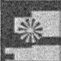
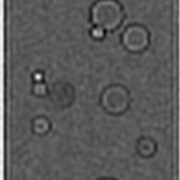
Reconstruction Gallery — 4 Scenes × 3 Scenarios
Method: CPU_baseline | Mismatch: nominal (nominal=True, perturbed=False)
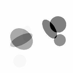
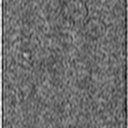
Ground Truth
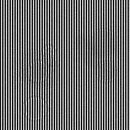
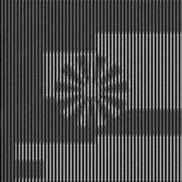
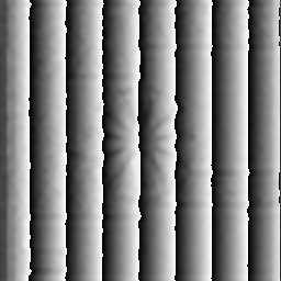
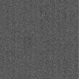
Measurement
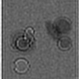
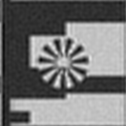
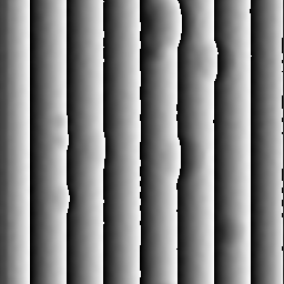
Reconstruction
Ground Truth
Measurement
Reconstruction
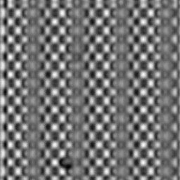
Ground Truth
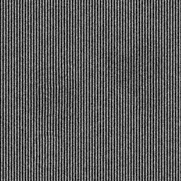
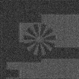
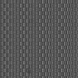
Measurement (perturbed)

Reconstruction


Mean PSNR Across All Scenes
Per-scene PSNR breakdown (4 scenes)
| Scene | I (PSNR) | I (SSIM) | II (PSNR) | II (SSIM) | III (PSNR) | III (SSIM) |
|---|---|---|---|---|---|---|
| scene_00 | 4.955552921136905 | 0.407475872520724 | 4.8344745201761 | 0.21817204737509321 | 5.3625136475527055 | 0.11097012672738123 |
| scene_01 | 11.849382664704038 | 0.31678578818849334 | 9.995445112699356 | 0.17336745505302376 | 4.800972769085293 | 0.04343594355266882 |
| scene_02 | 4.982413445816945 | 0.0938872975404209 | 4.317158116222904 | 0.10918194599808263 | 4.849174773211876 | 0.12794261561550066 |
| scene_03 | 4.121482528565731 | 0.37876904108358495 | 5.118790365277068 | 0.20783434716227533 | 5.072246662335454 | 0.11109208535878076 |
| Mean | 6.477207890055905 | 0.2992294998333058 | 6.0664670285938564 | 0.17713894889711873 | 5.021226963046332 | 0.09836019281358288 |
Experimental Setup
Key References
- Cuche et al., 'Digital holography for quantitative phase-contrast imaging', Optics Letters 24, 291-293 (1999)
- Kim, 'Principles and techniques of digital holographic microscopy', SPIE Reviews 1, 018005 (2010)
Canonical Datasets
- Lyncee Tec DHM application datasets
- HoloGAN benchmark (simulated holograms)
Spec DAG — Forward Model Pipeline
P(Fresnel) → D(g, η₁)
Mismatch Parameters
| Symbol | Parameter | Description | Nominal | Perturbed |
|---|---|---|---|---|
| Δλ | wavelength | Wavelength error (nm) | 0 | 0.5 |
| Δz | prop_distance | Propagation distance error (μm) | 0 | 5.0 |
| Δθ | tilt | Reference beam tilt (mrad) | 0 | 0.5 |
Credits System
Spec Primitives Reference (11 primitives)
Free-space or medium propagation kernel (Fresnel, Rayleigh-Sommerfeld).
Spatial or spatio-temporal amplitude modulation (coded aperture, SLM pattern).
Geometric projection operator (Radon transform, fan-beam, cone-beam).
Sampling in the Fourier / k-space domain (MRI, ptychography).
Shift-invariant convolution with a point-spread function (PSF).
Summation along a physical dimension (spectral, temporal, angular).
Sensor readout with gain g and noise model η (Gaussian, Poisson, mixed).
Patterned illumination (block, Hadamard, random) applied to the scene.
Spectral dispersion element (prism, grating) with shift α and aperture a.
Sample or gantry rotation (CT, electron tomography).
Spectral filter or monochromator selecting a wavelength band.