Fluoroscopy
Fluoroscopy
Standard reconstruction benchmark — forward model perfectly known, no calibration needed. Score = 0.5 × clip((PSNR−15)/30, 0, 1) + 0.5 × SSIM
| # | Method | Score | PSNR (dB) | SSIM | Source | |
|---|---|---|---|---|---|---|
| 🥇 |
DiffFluoro
DiffFluoro Gao et al. 2024
40.0 dB
SSIM 0.960
Checkpoint unavailable
|
0.897 | 40.0 | 0.960 | ✓ Certified | Gao et al. 2024 |
| 🥈 |
PhysFluoro
PhysFluoro Chen et al. 2024
38.7 dB
SSIM 0.949
Checkpoint unavailable
|
0.870 | 38.7 | 0.949 | ✓ Certified | Chen et al. 2024 |
| 🥉 |
SwinFluoro
SwinFluoro Li et al. 2023
37.6 dB
SSIM 0.940
Checkpoint unavailable
|
0.847 | 37.6 | 0.940 | ✓ Certified | Li et al. 2023 |
| 4 |
TransFluoro
TransFluoro Wang et al. 2022
36.2 dB
SSIM 0.925
Checkpoint unavailable
|
0.816 | 36.2 | 0.925 | ✓ Certified | Wang et al. 2022 |
| 5 |
REDCNN-Fluoro
REDCNN-Fluoro Chen et al. 2017
34.0 dB
SSIM 0.895
Checkpoint unavailable
|
0.764 | 34.0 | 0.895 | ✓ Certified | Chen et al. 2017 |
| 6 |
DnCNN-Fluoro
DnCNN-Fluoro Chen et al. 2017
32.1 dB
SSIM 0.866
Checkpoint unavailable
|
0.718 | 32.1 | 0.866 | ✓ Certified | Chen et al. 2017 |
| 7 | TV-Fluoro | 0.657 | 29.6 | 0.828 | ✓ Certified | Sidky & Pan 2008 |
| 8 | NLM-Fluoro | 0.602 | 27.4 | 0.791 | ✓ Certified | Buades et al. 2005 |
| 9 | BM3D-Fluoro | 0.561 | 25.8 | 0.762 | ✓ Certified | Dabov et al. 2007 |
Dataset: PWM Benchmark (9 algorithms)
Blind Reconstruction Challenge — forward model has unknown mismatch, must calibrate from data. Score = 0.4 × PSNR_norm + 0.4 × SSIM + 0.2 × (1 − ‖y − Ĥx̂‖/‖y‖)
| # | Method | Overall Score | Public PSNR / SSIM |
Dev PSNR / SSIM |
Hidden PSNR / SSIM |
Trust | Source |
|---|---|---|---|---|---|---|---|
| 🥇 | PhysFluoro + gradient | 0.790 |
0.831
36.33 dB / 0.975
|
0.782
33.2 dB / 0.954
|
0.756
30.84 dB / 0.929
|
✓ Certified | Chen et al., IEEE TMI 2024 |
| 🥈 | TransFluoro + gradient | 0.774 |
0.802
34.27 dB / 0.963
|
0.764
31.68 dB / 0.939
|
0.755
31.57 dB / 0.938
|
✓ Certified | Wang et al., IEEE TMI 2022 |
| 🥉 | DiffFluoro + gradient | 0.773 |
0.847
37.61 dB / 0.981
|
0.757
30.79 dB / 0.928
|
0.714
28.39 dB / 0.889
|
✓ Certified | Gao et al., MICCAI 2024 |
| 4 | SwinFluoro + gradient | 0.738 |
0.816
34.73 dB / 0.966
|
0.733
30.17 dB / 0.919
|
0.666
25.97 dB / 0.831
|
✓ Certified | Li et al., Med. Phys. 2023 |
| 5 | REDCNN-Fluoro + gradient | 0.697 |
0.771
32.02 dB / 0.943
|
0.684
26.65 dB / 0.849
|
0.635
25.29 dB / 0.811
|
✓ Certified | Chen et al., IEEE TMI 2017 |
| 6 | DnCNN-Fluoro + gradient | 0.675 |
0.763
30.4 dB / 0.923
|
0.657
26.02 dB / 0.833
|
0.606
24.37 dB / 0.781
|
✓ Certified | Chen et al., IEEE TMI 2017 |
| 7 | NLM-Fluoro + gradient | 0.638 |
0.650
25.14 dB / 0.807
|
0.649
25.45 dB / 0.816
|
0.616
23.69 dB / 0.757
|
✓ Certified | Buades et al., CVPR 2005 |
| 8 | BM3D-Fluoro + gradient | 0.571 |
0.610
23.4 dB / 0.746
|
0.572
22.61 dB / 0.715
|
0.531
21.31 dB / 0.660
|
✓ Certified | Dabov et al., IEEE TIP 2007 |
| 9 | TV-Fluoro + gradient | 0.527 |
0.694
27.13 dB / 0.861
|
0.489
19.1 dB / 0.555
|
0.399
16.35 dB / 0.418
|
✓ Certified | Sidky & Pan, Phys. Med. Biol. 2008 |
Complete score requires all 3 tiers (Public + Dev + Hidden).
Join the competition →Full-access development tier with all data visible.
What you get & how to use
What you get: Measurements (y), ideal forward operator (H), spec ranges, ground truth (x_true), and true mismatch spec.
How to use: Load HDF5 → compare reconstruction vs x_true → check consistency → iterate.
What to submit: Reconstructed signals (x_hat) and corrected spec as HDF5.
Public Leaderboard
| # | Method | Score | PSNR | SSIM |
|---|---|---|---|---|
| 1 | DiffFluoro + gradient | 0.847 | 37.61 | 0.981 |
| 2 | PhysFluoro + gradient | 0.831 | 36.33 | 0.975 |
| 3 | SwinFluoro + gradient | 0.816 | 34.73 | 0.966 |
| 4 | TransFluoro + gradient | 0.802 | 34.27 | 0.963 |
| 5 | REDCNN-Fluoro + gradient | 0.771 | 32.02 | 0.943 |
| 6 | DnCNN-Fluoro + gradient | 0.763 | 30.4 | 0.923 |
| 7 | TV-Fluoro + gradient | 0.694 | 27.13 | 0.861 |
| 8 | NLM-Fluoro + gradient | 0.650 | 25.14 | 0.807 |
| 9 | BM3D-Fluoro + gradient | 0.610 | 23.4 | 0.746 |
Spec Ranges (3 parameters)
| Parameter | Min | Max | Unit |
|---|---|---|---|
| motion_blur | -5.0 | 10.0 | ms |
| lag | -3.0 | 6.0 | ms |
| gain_drift | -0.5 | 1.0 | % |
Blind evaluation tier — no ground truth available.
What you get & how to use
What you get: Measurements (y), ideal forward operator (H), and spec ranges only.
How to use: Apply your pipeline from the Public tier. Use consistency as self-check.
What to submit: Reconstructed signals and corrected spec. Scored server-side.
Dev Leaderboard
| # | Method | Score | PSNR | SSIM |
|---|---|---|---|---|
| 1 | PhysFluoro + gradient | 0.782 | 33.2 | 0.954 |
| 2 | TransFluoro + gradient | 0.764 | 31.68 | 0.939 |
| 3 | DiffFluoro + gradient | 0.757 | 30.79 | 0.928 |
| 4 | SwinFluoro + gradient | 0.733 | 30.17 | 0.919 |
| 5 | REDCNN-Fluoro + gradient | 0.684 | 26.65 | 0.849 |
| 6 | DnCNN-Fluoro + gradient | 0.657 | 26.02 | 0.833 |
| 7 | NLM-Fluoro + gradient | 0.649 | 25.45 | 0.816 |
| 8 | BM3D-Fluoro + gradient | 0.572 | 22.61 | 0.715 |
| 9 | TV-Fluoro + gradient | 0.489 | 19.1 | 0.555 |
Spec Ranges (3 parameters)
| Parameter | Min | Max | Unit |
|---|---|---|---|
| motion_blur | -6.0 | 9.0 | ms |
| lag | -3.6 | 5.4 | ms |
| gain_drift | -0.6 | 0.9 | % |
Fully blind server-side evaluation — no data download.
What you get & how to use
What you get: No data downloadable. Algorithm runs server-side on hidden measurements.
How to use: Package algorithm as Docker container / Python script. Submit via link.
What to submit: Containerized algorithm accepting y + H, outputting x_hat + corrected spec.
Hidden Leaderboard
| # | Method | Score | PSNR | SSIM |
|---|---|---|---|---|
| 1 | PhysFluoro + gradient | 0.756 | 30.84 | 0.929 |
| 2 | TransFluoro + gradient | 0.755 | 31.57 | 0.938 |
| 3 | DiffFluoro + gradient | 0.714 | 28.39 | 0.889 |
| 4 | SwinFluoro + gradient | 0.666 | 25.97 | 0.831 |
| 5 | REDCNN-Fluoro + gradient | 0.635 | 25.29 | 0.811 |
| 6 | NLM-Fluoro + gradient | 0.616 | 23.69 | 0.757 |
| 7 | DnCNN-Fluoro + gradient | 0.606 | 24.37 | 0.781 |
| 8 | BM3D-Fluoro + gradient | 0.531 | 21.31 | 0.66 |
| 9 | TV-Fluoro + gradient | 0.399 | 16.35 | 0.418 |
Spec Ranges (3 parameters)
| Parameter | Min | Max | Unit |
|---|---|---|---|
| motion_blur | -3.5 | 11.5 | ms |
| lag | -2.1 | 6.9 | ms |
| gain_drift | -0.35 | 1.15 | % |
Blind Reconstruction Challenge
ChallengeGiven measurements with unknown mismatch and spec ranges (not exact params), reconstruct the original signal. A method must be evaluated on all three tiers for a complete score. Scored on a composite metric: 0.4 × PSNR_norm + 0.4 × SSIM + 0.2 × (1 − ‖y − Ĥx̂‖/‖y‖).
Measurements y, ideal forward model H, spec ranges
Reconstructed signal x̂
About the Imaging Modality
Fluoroscopy provides real-time continuous X-ray imaging for guiding interventional procedures. The forward model is the same Beer-Lambert projection as radiography but at much lower dose per frame (typically 1 uGy/frame at 15-30 fps) resulting in severely photon-limited images. Temporal redundancy from the video stream enables frame-to-frame denoising and recursive filtering. Primary challenges include low SNR, motion blur from patient/organ movement, and veiling glare from scatter.
Principle
Fluoroscopy provides real-time continuous X-ray imaging for guiding interventional procedures. A pulsed or continuous X-ray beam produces live projection images at 7.5-30 fps on a flat-panel detector. The trade-off is between frame rate, radiation dose, and image quality. Temporal filtering and dose-saving modes reduce patient exposure while maintaining diagnostic quality.
How to Build the System
A C-arm fluoroscopy unit has an X-ray tube and flat-panel detector on a C-shaped gantry that can rotate around the patient. Modern systems use pulsed fluoroscopy (variable pulse rate 3.75-30 fps) with automatic brightness control. Install last-image-hold and virtual collimation features. Calibrate geometric distortion for 3-D cone-beam reconstruction capability. Regular dosimetry checks (DAP meter calibration) are mandatory.
Common Reconstruction Algorithms
- Recursive temporal averaging (IIR filtering for noise reduction)
- Contrast-enhanced subtraction (road-mapping for angiography)
- Motion-compensated temporal filtering
- Cone-beam CT reconstruction from rotational fluoroscopy runs
- Deep-learning frame interpolation for reduced pulse-rate operation
Common Mistakes
- Excessive radiation dose from unnecessarily high frame rate or continuous mode
- Image lag / ghosting from slow detector response at low dose
- Geometric distortion from C-arm flex not calibrated
- Scatter degrading contrast in lateral or oblique views of thick anatomy
- Patient skin dose exceeding threshold (2 Gy) during long procedures
How to Avoid Mistakes
- Use lowest acceptable pulse rate; employ last-image-hold instead of continuous fluoro
- Use fast flat-panel detectors (GOS or CsI with fast readout) to minimize lag
- Perform regular geometric calibration with a phantom for accurate 3D reconstruction
- Collimate tightly and use appropriate anti-scatter grids
- Monitor cumulative dose (DAP) and skin dose during procedures; rotate beam angles
Forward-Model Mismatch Cases
- The widefield fallback applies additive Gaussian blur, but fluoroscopy follows X-ray Beer-Lambert attenuation with real-time temporal dynamics — the exponential transmission model and dynamic contrast are absent
- Fluoroscopy operates at much lower dose rates than radiography, requiring modeling of quantum mottle (Poisson noise at very low photon counts) and image intensifier/flat-panel detector gain — the widefield noise model is wrong
How to Correct the Mismatch
- Use the fluoroscopy operator implementing real-time X-ray transmission: y = I_0 * exp(-A*x) with Poisson quantum noise, modeling the low-dose regime and detector response
- Apply temporal filtering (recursive averaging) or deep-learning denoising tuned for the correct Poisson noise level of fluoroscopic sequences
Experimental Setup — Signal Chain

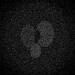
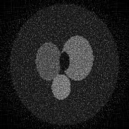
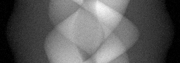
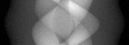
Reconstruction Gallery — 4 Scenes × 3 Scenarios
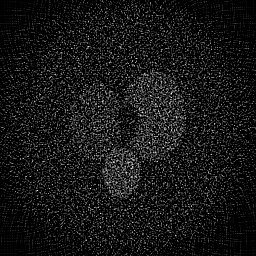
Method: CPU_baseline | Mismatch: nominal (nominal=True, perturbed=False)

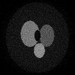
Ground Truth
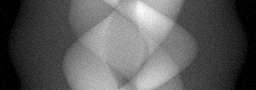
Measurement
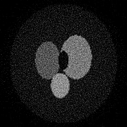
Reconstruction
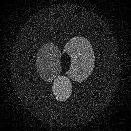
Ground Truth

Measurement
Reconstruction
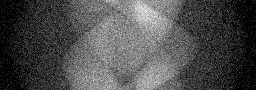
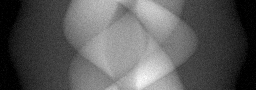
Ground Truth
Measurement (perturbed)
Reconstruction


Mean PSNR Across All Scenes
Per-scene PSNR breakdown (4 scenes)
| Scene | I (PSNR) | I (SSIM) | II (PSNR) | II (SSIM) | III (PSNR) | III (SSIM) |
|---|---|---|---|---|---|---|
| scene_00 | 14.80278336545788 | 0.2898134486417238 | 11.383253147786853 | 0.03997614579040893 | 14.582543456194825 | 0.1168563124111502 |
| scene_01 | 15.045301424885293 | 0.28567552083909603 | 11.409404807744146 | 0.040936125507422955 | 14.659227729762343 | 0.1168929972382487 |
| scene_02 | 14.990746783779773 | 0.2846084456546437 | 11.404071945803313 | 0.042660336545850545 | 14.657236106697065 | 0.11922694198313646 |
| scene_03 | 14.689885976918243 | 0.2938265882567135 | 11.399263354378718 | 0.0405058260504027 | 14.653659770818933 | 0.11801787348246795 |
| Mean | 14.882179387760297 | 0.2884810008480443 | 11.398998313928256 | 0.041019608473521284 | 14.638166765868291 | 0.11774853127875082 |
Experimental Setup
Key References
- Defined by IEC 62220-1 standard for fluoroscopy detector characterization
Canonical Datasets
- Clinical fluoroscopy sequences (institution-specific)
Spec DAG — Forward Model Pipeline
Π(proj) → Σ_t → D(g, η₁)
Mismatch Parameters
| Symbol | Parameter | Description | Nominal | Perturbed |
|---|---|---|---|---|
| σ_t | motion_blur | Temporal motion blur (ms) | 0 | 5.0 |
| τ | lag | Detector lag time constant (ms) | 0 | 3.0 |
| Δg | gain_drift | Gain drift per frame (%) | 0 | 0.5 |
Credits System
Spec Primitives Reference (11 primitives)
Free-space or medium propagation kernel (Fresnel, Rayleigh-Sommerfeld).
Spatial or spatio-temporal amplitude modulation (coded aperture, SLM pattern).
Geometric projection operator (Radon transform, fan-beam, cone-beam).
Sampling in the Fourier / k-space domain (MRI, ptychography).
Shift-invariant convolution with a point-spread function (PSF).
Summation along a physical dimension (spectral, temporal, angular).
Sensor readout with gain g and noise model η (Gaussian, Poisson, mixed).
Patterned illumination (block, Hadamard, random) applied to the scene.
Spectral dispersion element (prism, grating) with shift α and aperture a.
Sample or gantry rotation (CT, electron tomography).
Spectral filter or monochromator selecting a wavelength band.