Electron Holography
Electron Holography
Standard reconstruction benchmark — forward model perfectly known, no calibration needed. Score = 0.5 × clip((PSNR−15)/30, 0, 1) + 0.5 × SSIM
| # | Method | Score | PSNR (dB) | SSIM | Source | |
|---|---|---|---|---|---|---|
| 🥇 |
DiffHolo
DiffHolo Gao et al. 2024
39.2 dB
SSIM 0.953
Checkpoint unavailable
|
0.880 | 39.2 | 0.953 | ✓ Certified | Gao et al. 2024 |
| 🥈 |
PhysHolo
PhysHolo Chen et al. 2024
37.8 dB
SSIM 0.942
Checkpoint unavailable
|
0.851 | 37.8 | 0.942 | ✓ Certified | Chen et al. 2024 |
| 🥉 |
SwinHolo
SwinHolo Wang et al. 2023
36.5 dB
SSIM 0.931
Checkpoint unavailable
|
0.824 | 36.5 | 0.931 | ✓ Certified | Wang et al. 2023 |
| 4 |
TransHolo
TransHolo Li et al. 2022
34.9 dB
SSIM 0.913
Checkpoint unavailable
|
0.788 | 34.9 | 0.913 | ✓ Certified | Li et al. 2022 |
| 5 |
DeepHolo
DeepHolo Rivenson et al. 2018
32.4 dB
SSIM 0.875
Checkpoint unavailable
|
0.728 | 32.4 | 0.875 | ✓ Certified | Rivenson et al. 2018 |
| 6 |
DnCNN-Holo
DnCNN-Holo Gao et al. 2019
29.6 dB
SSIM 0.835
Checkpoint unavailable
|
0.661 | 29.6 | 0.835 | ✓ Certified | Gao et al. 2019 |
| 7 | TV-Phase | 0.588 | 26.8 | 0.783 | ✓ Certified | Beleggia et al. 2004 |
| 8 | WDD-Holo | 0.524 | 24.2 | 0.742 | ✓ Certified | Lichte 1986 |
| 9 | FFT-Holo | 0.458 | 21.5 | 0.700 | ✓ Certified | Lehmann & Lichte 2002 |
Dataset: PWM Benchmark (9 algorithms)
Blind Reconstruction Challenge — forward model has unknown mismatch, must calibrate from data. Score = 0.4 × PSNR_norm + 0.4 × SSIM + 0.2 × (1 − ‖y − Ĥx̂‖/‖y‖)
| # | Method | Overall Score | Public PSNR / SSIM |
Dev PSNR / SSIM |
Hidden PSNR / SSIM |
Trust | Source |
|---|---|---|---|---|---|---|---|
| 🥇 | SwinHolo + gradient | 0.751 |
0.826
35.37 dB / 0.970
|
0.742
30.87 dB / 0.929
|
0.685
26.88 dB / 0.855
|
✓ Certified | Wang et al., Ultramicroscopy 2023 |
| 🥈 | DiffHolo + gradient | 0.742 |
0.837
37.02 dB / 0.978
|
0.730
30.21 dB / 0.920
|
0.659
26.79 dB / 0.853
|
✓ Certified | Gao et al., NeurIPS 2024 |
| 🥉 | PhysHolo + gradient | 0.737 |
0.841
36.49 dB / 0.976
|
0.704
28.67 dB / 0.894
|
0.667
26.11 dB / 0.835
|
✓ Certified | Chen et al., Nat. Commun. 2024 |
| 4 | TransHolo + gradient | 0.721 |
0.805
33.44 dB / 0.956
|
0.718
29.09 dB / 0.902
|
0.640
25.5 dB / 0.818
|
✓ Certified | Li et al., Nat. Commun. 2022 |
| 5 | DeepHolo + gradient | 0.678 |
0.768
30.99 dB / 0.931
|
0.661
25.56 dB / 0.819
|
0.606
23.46 dB / 0.749
|
✓ Certified | Rivenson et al., Optica 2018 |
| 6 | DnCNN-Holo + gradient | 0.634 |
0.727
28.57 dB / 0.892
|
0.603
23.58 dB / 0.753
|
0.571
22.5 dB / 0.711
|
✓ Certified | Gao et al., Ultramicroscopy 2019 |
| 7 | WDD-Holo + gradient | 0.530 |
0.610
23.14 dB / 0.737
|
0.504
19.75 dB / 0.587
|
0.475
18.78 dB / 0.539
|
✓ Certified | Lichte, Ultramicroscopy 1986 |
| 8 | TV-Phase + gradient | 0.530 |
0.668
25.5 dB / 0.818
|
0.501
19.97 dB / 0.597
|
0.420
17.73 dB / 0.487
|
✓ Certified | Beleggia et al., Ultramicroscopy 2004 |
| 9 | FFT-Holo + gradient | 0.459 |
0.534
20.28 dB / 0.612
|
0.440
17.54 dB / 0.477
|
0.403
16.31 dB / 0.416
|
✓ Certified | Lehmann & Lichte, Microsc. Microanal. 2002 |
Complete score requires all 3 tiers (Public + Dev + Hidden).
Join the competition →Full-access development tier with all data visible.
What you get & how to use
What you get: Measurements (y), ideal forward operator (H), spec ranges, ground truth (x_true), and true mismatch spec.
How to use: Load HDF5 → compare reconstruction vs x_true → check consistency → iterate.
What to submit: Reconstructed signals (x_hat) and corrected spec as HDF5.
Public Leaderboard
| # | Method | Score | PSNR | SSIM |
|---|---|---|---|---|
| 1 | PhysHolo + gradient | 0.841 | 36.49 | 0.976 |
| 2 | DiffHolo + gradient | 0.837 | 37.02 | 0.978 |
| 3 | SwinHolo + gradient | 0.826 | 35.37 | 0.97 |
| 4 | TransHolo + gradient | 0.805 | 33.44 | 0.956 |
| 5 | DeepHolo + gradient | 0.768 | 30.99 | 0.931 |
| 6 | DnCNN-Holo + gradient | 0.727 | 28.57 | 0.892 |
| 7 | TV-Phase + gradient | 0.668 | 25.5 | 0.818 |
| 8 | WDD-Holo + gradient | 0.610 | 23.14 | 0.737 |
| 9 | FFT-Holo + gradient | 0.534 | 20.28 | 0.612 |
Spec Ranges (3 parameters)
| Parameter | Min | Max | Unit |
|---|---|---|---|
| biprism_voltage | -2.0 | 4.0 | V |
| fringe_spacing | -0.1 | 0.2 | nm |
| partial_coherence | -5.0 | 10.0 | % |
Blind evaluation tier — no ground truth available.
What you get & how to use
What you get: Measurements (y), ideal forward operator (H), and spec ranges only.
How to use: Apply your pipeline from the Public tier. Use consistency as self-check.
What to submit: Reconstructed signals and corrected spec. Scored server-side.
Dev Leaderboard
| # | Method | Score | PSNR | SSIM |
|---|---|---|---|---|
| 1 | SwinHolo + gradient | 0.742 | 30.87 | 0.929 |
| 2 | DiffHolo + gradient | 0.730 | 30.21 | 0.92 |
| 3 | TransHolo + gradient | 0.718 | 29.09 | 0.902 |
| 4 | PhysHolo + gradient | 0.704 | 28.67 | 0.894 |
| 5 | DeepHolo + gradient | 0.661 | 25.56 | 0.819 |
| 6 | DnCNN-Holo + gradient | 0.603 | 23.58 | 0.753 |
| 7 | WDD-Holo + gradient | 0.504 | 19.75 | 0.587 |
| 8 | TV-Phase + gradient | 0.501 | 19.97 | 0.597 |
| 9 | FFT-Holo + gradient | 0.440 | 17.54 | 0.477 |
Spec Ranges (3 parameters)
| Parameter | Min | Max | Unit |
|---|---|---|---|
| biprism_voltage | -2.4 | 3.6 | V |
| fringe_spacing | -0.12 | 0.18 | nm |
| partial_coherence | -6.0 | 9.0 | % |
Fully blind server-side evaluation — no data download.
What you get & how to use
What you get: No data downloadable. Algorithm runs server-side on hidden measurements.
How to use: Package algorithm as Docker container / Python script. Submit via link.
What to submit: Containerized algorithm accepting y + H, outputting x_hat + corrected spec.
Hidden Leaderboard
| # | Method | Score | PSNR | SSIM |
|---|---|---|---|---|
| 1 | SwinHolo + gradient | 0.685 | 26.88 | 0.855 |
| 2 | PhysHolo + gradient | 0.667 | 26.11 | 0.835 |
| 3 | DiffHolo + gradient | 0.659 | 26.79 | 0.853 |
| 4 | TransHolo + gradient | 0.640 | 25.5 | 0.818 |
| 5 | DeepHolo + gradient | 0.606 | 23.46 | 0.749 |
| 6 | DnCNN-Holo + gradient | 0.571 | 22.5 | 0.711 |
| 7 | WDD-Holo + gradient | 0.475 | 18.78 | 0.539 |
| 8 | TV-Phase + gradient | 0.420 | 17.73 | 0.487 |
| 9 | FFT-Holo + gradient | 0.403 | 16.31 | 0.416 |
Spec Ranges (3 parameters)
| Parameter | Min | Max | Unit |
|---|---|---|---|
| biprism_voltage | -1.4 | 4.6 | V |
| fringe_spacing | -0.07 | 0.23 | nm |
| partial_coherence | -3.5 | 11.5 | % |
Blind Reconstruction Challenge
ChallengeGiven measurements with unknown mismatch and spec ranges (not exact params), reconstruct the original signal. A method must be evaluated on all three tiers for a complete score. Scored on a composite metric: 0.4 × PSNR_norm + 0.4 × SSIM + 0.2 × (1 − ‖y − Ĥx̂‖/‖y‖).
Measurements y, ideal forward model H, spec ranges
Reconstructed signal x̂
About the Imaging Modality
Off-axis electron holography records the interference pattern between an object wave (passed through the specimen) and a reference wave (passed through vacuum) using an electrostatic biprism. The hologram encodes the phase shift imparted by electric and magnetic fields within the specimen. Fourier filtering isolates the sideband carrying the complex wave information, from which amplitude and phase are extracted. Phase sensitivity of ~2*pi/1000 enables mapping of nanoscale electric and magnetic fields in materials.
Principle
Electron holography uses the interference between an object wave (transmitted through the specimen) and a reference wave (passing through vacuum) to record both amplitude and phase of the electron wave. An electrostatic biprism (charged wire) deflects the two waves to overlap and form interference fringes. Numerical reconstruction recovers the phase shift, which is sensitive to electrostatic potentials and magnetic fields in the specimen.
How to Build the System
Use a TEM (≥200 kV, FEG source for high coherence) equipped with an electron biprism (a thin metallized quartz fiber at adjustable voltage 50-300 V). Position the specimen so one half of the biprism overlaps the specimen edge and the other half is in vacuum. Record the hologram on a direct-electron detector. Fringe spacing should be 3-4× the desired resolution. Acquire reference holograms (empty) for normalization.
Common Reconstruction Algorithms
- Fourier filtering (sideband extraction and inverse FFT for phase/amplitude)
- Phase unwrapping for large phase shifts (>2π)
- Mean inner potential measurement from phase maps
- Magnetic induction mapping (from phase gradient of Lorentz holography)
- In-line holography (through-focus series) with transport-of-intensity equation
Common Mistakes
- Biprism voltage too low, giving insufficient overlap and poor fringe contrast
- Fresnel fringes from specimen edge contaminating the holographic fringes
- Not acquiring and dividing by a reference hologram, leaving biprism distortions
- Specimen too thick, reducing fringe visibility from inelastic scattering
- Stray magnetic fields causing unwanted phase shifts in the reference wave
How to Avoid Mistakes
- Optimize biprism voltage for 3-4× oversampling of desired resolution with good contrast
- Extend vacuum reference beyond the specimen edge; mask Fresnel fringe regions
- Always acquire reference holograms and compute the normalized phase
- Use thin specimens (< 50-80 nm) to maintain fringe contrast above 10%
- Enclose the TEM column in mu-metal shielding; degauss the objective lens for Lorentz mode
Forward-Model Mismatch Cases
- The widefield fallback produces real-valued output, but electron holography records the interference between object and reference electron waves — the complex-valued hologram encodes electromagnetic potentials (electric and magnetic fields) inside the specimen via the Aharonov-Bohm phase shift
- The biprism interference fringes encode quantitative phase information (phase shift = C_E * integral(V(x,y,z)dz) for electrostatic, and -(e/hbar) * integral(A*dl) for magnetic) — the widefield blur destroys fringe contrast and all phase information
How to Correct the Mismatch
- Use the electron holography operator that models biprism-mediated interference between object wave (with Aharonov-Bohm phase shift) and vacuum reference wave, producing complex holographic fringes
- Reconstruct phase maps using Fourier sideband filtering and inverse FFT; for magnetic specimens, use Lorentz mode and separate electrostatic and magnetic phase contributions
Experimental Setup — Signal Chain

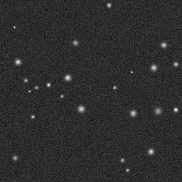
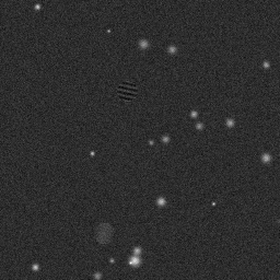
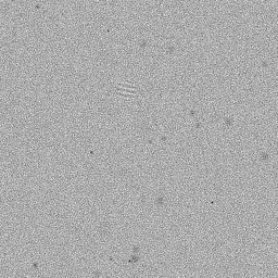
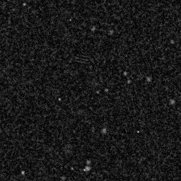
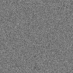
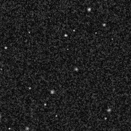
Reconstruction Gallery — 4 Scenes × 3 Scenarios
Method: CPU_baseline | Mismatch: nominal (nominal=True, perturbed=False)
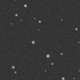
Ground Truth
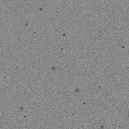
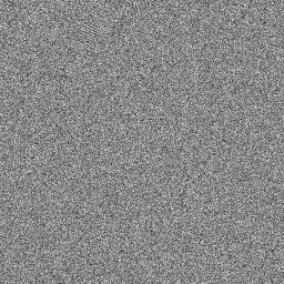
Measurement
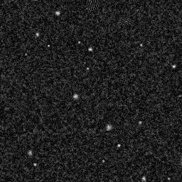
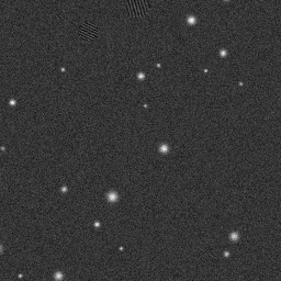
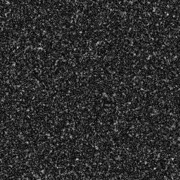
Reconstruction
Ground Truth
Measurement
Reconstruction
Ground Truth
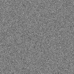
Measurement (perturbed)
Reconstruction
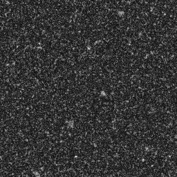
Mean PSNR Across All Scenes
Per-scene PSNR breakdown (4 scenes)
| Scene | I (PSNR) | I (SSIM) | II (PSNR) | II (SSIM) | III (PSNR) | III (SSIM) |
|---|---|---|---|---|---|---|
| scene_00 | 19.401488157362497 | 0.48886704895877836 | 16.857966791337656 | 0.08915507096515726 | 19.015339082048712 | 0.19323876033569679 |
| scene_01 | 20.386994971632934 | 0.49771035050842166 | 17.188182006293506 | 0.08456095595654231 | 19.00326347865052 | 0.1825080566719887 |
| scene_02 | 20.109288125342772 | 0.4612187812713385 | 17.552917796407378 | 0.08129459333217216 | 19.721316784917846 | 0.17921822573660165 |
| scene_03 | 19.33896725172696 | 0.48831334454774855 | 16.902556624008536 | 0.09105537055754624 | 18.83727554088228 | 0.1898195007747968 |
| Mean | 19.80918462651629 | 0.48402738132157175 | 17.125405804511768 | 0.0865164977028545 | 19.144298721624843 | 0.186196135879771 |
Experimental Setup
Key References
- Dunin-Borkowski et al., 'Electron holography of nanostructured materials', Encyclopedia of Nanoscience and Nanotechnology (2004)
- Lichte & Lehmann, 'Electron holography — basics and applications', Rep. Prog. Phys. 71, 016102 (2008)
Canonical Datasets
- Holography benchmark datasets (Forschungszentrum Julich)
Spec DAG — Forward Model Pipeline
P(e⁻) → Σ(interference) → D(g, η₁)
Mismatch Parameters
| Symbol | Parameter | Description | Nominal | Perturbed |
|---|---|---|---|---|
| ΔV_b | biprism_voltage | Biprism voltage error (V) | 0 | 2.0 |
| Δd_f | fringe_spacing | Fringe spacing error (nm) | 0 | 0.1 |
| Δμ | partial_coherence | Spatial coherence error (%) | 0 | 5.0 |
Credits System
Spec Primitives Reference (11 primitives)
Free-space or medium propagation kernel (Fresnel, Rayleigh-Sommerfeld).
Spatial or spatio-temporal amplitude modulation (coded aperture, SLM pattern).
Geometric projection operator (Radon transform, fan-beam, cone-beam).
Sampling in the Fourier / k-space domain (MRI, ptychography).
Shift-invariant convolution with a point-spread function (PSF).
Summation along a physical dimension (spectral, temporal, angular).
Sensor readout with gain g and noise model η (Gaussian, Poisson, mixed).
Patterned illumination (block, Hadamard, random) applied to the scene.
Spectral dispersion element (prism, grating) with shift α and aperture a.
Sample or gantry rotation (CT, electron tomography).
Spectral filter or monochromator selecting a wavelength band.