EELS
Electron Energy Loss Spectroscopy
Standard reconstruction benchmark — forward model perfectly known, no calibration needed. Score = 0.5 × clip((PSNR−15)/30, 0, 1) + 0.5 × SSIM
| # | Method | Score | PSNR (dB) | SSIM | Source | |
|---|---|---|---|---|---|---|
| 🥇 |
DiffEELS
DiffEELS Gao et al. 2024
39.3 dB
SSIM 0.954
Checkpoint unavailable
|
0.882 | 39.3 | 0.954 | ✓ Certified | Gao et al. 2024 |
| 🥈 |
PhysEELS
PhysEELS Chen et al. 2024
37.9 dB
SSIM 0.942
Checkpoint unavailable
|
0.853 | 37.9 | 0.942 | ✓ Certified | Chen et al. 2024 |
| 🥉 |
SwinEELS
SwinEELS Wang et al. 2023
36.7 dB
SSIM 0.932
Checkpoint unavailable
|
0.828 | 36.7 | 0.932 | ✓ Certified | Wang et al. 2023 |
| 4 |
TransEELS
TransEELS Li et al. 2022
35.1 dB
SSIM 0.915
Checkpoint unavailable
|
0.792 | 35.1 | 0.915 | ✓ Certified | Li et al. 2022 |
| 5 |
N2V-EELS
N2V-EELS Krull et al. 2019
32.6 dB
SSIM 0.876
Checkpoint unavailable
|
0.731 | 32.6 | 0.876 | ✓ Certified | Krull et al. 2019 |
| 6 |
DnCNN-EELS
DnCNN-EELS Kovarik et al. 2016
30.0 dB
SSIM 0.838
Checkpoint unavailable
|
0.669 | 30.0 | 0.838 | ✓ Certified | Kovarik et al. 2016 |
| 7 | ICA-EELS | 0.595 | 27.1 | 0.786 | ✓ Certified | Bosman et al. 2006 |
| 8 | MLS-EELS | 0.530 | 24.5 | 0.744 | ✓ Certified | Verbeeck & Van Aert 2004 |
| 9 | PowerLaw-EELS | 0.463 | 21.8 | 0.699 | ✓ Certified | Egerton 2011 |
Dataset: PWM Benchmark (9 algorithms)
Blind Reconstruction Challenge — forward model has unknown mismatch, must calibrate from data. Score = 0.4 × PSNR_norm + 0.4 × SSIM + 0.2 × (1 − ‖y − Ĥx̂‖/‖y‖)
| # | Method | Overall Score | Public PSNR / SSIM |
Dev PSNR / SSIM |
Hidden PSNR / SSIM |
Trust | Source |
|---|---|---|---|---|---|---|---|
| 🥇 | SwinEELS + gradient | 0.773 |
0.806
34.4 dB / 0.964
|
0.767
31.84 dB / 0.941
|
0.745
31.06 dB / 0.932
|
✓ Certified | Wang et al., npj Comput. Mater. 2023 |
| 🥈 | PhysEELS + gradient | 0.768 |
0.842
36.71 dB / 0.977
|
0.739
30.78 dB / 0.928
|
0.722
28.85 dB / 0.898
|
✓ Certified | Chen et al., Microsc. Microanal. 2024 |
| 🥉 | DiffEELS + gradient | 0.751 |
0.859
37.82 dB / 0.981
|
0.739
30.29 dB / 0.921
|
0.654
26.34 dB / 0.841
|
✓ Certified | Gao et al., NeurIPS 2024 |
| 4 | TransEELS + gradient | 0.743 |
0.783
32.29 dB / 0.946
|
0.752
31.47 dB / 0.937
|
0.694
28.56 dB / 0.892
|
✓ Certified | Li et al., Ultramicroscopy 2022 |
| 5 | N2V-EELS + gradient | 0.640 |
0.744
29.72 dB / 0.912
|
0.612
23.43 dB / 0.748
|
0.563
22.1 dB / 0.694
|
✓ Certified | Krull et al., NeurIPS 2019 |
| 6 | DnCNN-EELS + gradient | 0.566 |
0.733
28.93 dB / 0.899
|
0.517
20.17 dB / 0.607
|
0.448
18.4 dB / 0.520
|
✓ Certified | Kovarik et al., npj Comput. Mater. 2016 |
| 7 | PowerLaw-EELS + gradient | 0.482 |
0.488
18.87 dB / 0.543
|
0.485
19.02 dB / 0.551
|
0.474
18.73 dB / 0.536
|
✓ Certified | Egerton, EELS in the EM, Springer 2011 |
| 8 | MLS-EELS + gradient | 0.471 |
0.612
23.06 dB / 0.733
|
0.429
17.62 dB / 0.481
|
0.372
16.0 dB / 0.401
|
✓ Certified | Verbeeck & Van Aert, Ultramicroscopy 2004 |
| 9 | ICA-EELS + gradient | 0.456 |
0.645
24.94 dB / 0.800
|
0.412
16.92 dB / 0.446
|
0.310
13.77 dB / 0.300
|
✓ Certified | Bosman et al., Ultramicroscopy 2006 |
Complete score requires all 3 tiers (Public + Dev + Hidden).
Join the competition →Full-access development tier with all data visible.
What you get & how to use
What you get: Measurements (y), ideal forward operator (H), spec ranges, ground truth (x_true), and true mismatch spec.
How to use: Load HDF5 → compare reconstruction vs x_true → check consistency → iterate.
What to submit: Reconstructed signals (x_hat) and corrected spec as HDF5.
Public Leaderboard
| # | Method | Score | PSNR | SSIM |
|---|---|---|---|---|
| 1 | DiffEELS + gradient | 0.859 | 37.82 | 0.981 |
| 2 | PhysEELS + gradient | 0.842 | 36.71 | 0.977 |
| 3 | SwinEELS + gradient | 0.806 | 34.4 | 0.964 |
| 4 | TransEELS + gradient | 0.783 | 32.29 | 0.946 |
| 5 | N2V-EELS + gradient | 0.744 | 29.72 | 0.912 |
| 6 | DnCNN-EELS + gradient | 0.733 | 28.93 | 0.899 |
| 7 | ICA-EELS + gradient | 0.645 | 24.94 | 0.8 |
| 8 | MLS-EELS + gradient | 0.612 | 23.06 | 0.733 |
| 9 | PowerLaw-EELS + gradient | 0.488 | 18.87 | 0.543 |
Spec Ranges (3 parameters)
| Parameter | Min | Max | Unit |
|---|---|---|---|
| energy_dispersion | -0.002 | 0.004 | eV/channel |
| zero_loss_shift | -0.3 | 0.6 | eV |
| aberration | -2.0 | 4.0 | % |
Blind evaluation tier — no ground truth available.
What you get & how to use
What you get: Measurements (y), ideal forward operator (H), and spec ranges only.
How to use: Apply your pipeline from the Public tier. Use consistency as self-check.
What to submit: Reconstructed signals and corrected spec. Scored server-side.
Dev Leaderboard
| # | Method | Score | PSNR | SSIM |
|---|---|---|---|---|
| 1 | SwinEELS + gradient | 0.767 | 31.84 | 0.941 |
| 2 | TransEELS + gradient | 0.752 | 31.47 | 0.937 |
| 3 | PhysEELS + gradient | 0.739 | 30.78 | 0.928 |
| 4 | DiffEELS + gradient | 0.739 | 30.29 | 0.921 |
| 5 | N2V-EELS + gradient | 0.612 | 23.43 | 0.748 |
| 6 | DnCNN-EELS + gradient | 0.517 | 20.17 | 0.607 |
| 7 | PowerLaw-EELS + gradient | 0.485 | 19.02 | 0.551 |
| 8 | MLS-EELS + gradient | 0.429 | 17.62 | 0.481 |
| 9 | ICA-EELS + gradient | 0.412 | 16.92 | 0.446 |
Spec Ranges (3 parameters)
| Parameter | Min | Max | Unit |
|---|---|---|---|
| energy_dispersion | -0.0024 | 0.0036 | eV/channel |
| zero_loss_shift | -0.36 | 0.54 | eV |
| aberration | -2.4 | 3.6 | % |
Fully blind server-side evaluation — no data download.
What you get & how to use
What you get: No data downloadable. Algorithm runs server-side on hidden measurements.
How to use: Package algorithm as Docker container / Python script. Submit via link.
What to submit: Containerized algorithm accepting y + H, outputting x_hat + corrected spec.
Hidden Leaderboard
| # | Method | Score | PSNR | SSIM |
|---|---|---|---|---|
| 1 | SwinEELS + gradient | 0.745 | 31.06 | 0.932 |
| 2 | PhysEELS + gradient | 0.722 | 28.85 | 0.898 |
| 3 | TransEELS + gradient | 0.694 | 28.56 | 0.892 |
| 4 | DiffEELS + gradient | 0.654 | 26.34 | 0.841 |
| 5 | N2V-EELS + gradient | 0.563 | 22.1 | 0.694 |
| 6 | PowerLaw-EELS + gradient | 0.474 | 18.73 | 0.536 |
| 7 | DnCNN-EELS + gradient | 0.448 | 18.4 | 0.52 |
| 8 | MLS-EELS + gradient | 0.372 | 16.0 | 0.401 |
| 9 | ICA-EELS + gradient | 0.310 | 13.77 | 0.3 |
Spec Ranges (3 parameters)
| Parameter | Min | Max | Unit |
|---|---|---|---|
| energy_dispersion | -0.0014 | 0.0046 | eV/channel |
| zero_loss_shift | -0.21 | 0.69 | eV |
| aberration | -1.4 | 4.6 | % |
Blind Reconstruction Challenge
ChallengeGiven measurements with unknown mismatch and spec ranges (not exact params), reconstruct the original signal. A method must be evaluated on all three tiers for a complete score. Scored on a composite metric: 0.4 × PSNR_norm + 0.4 × SSIM + 0.2 × (1 − ‖y − Ĥx̂‖/‖y‖).
Measurements y, ideal forward model H, spec ranges
Reconstructed signal x̂
About the Imaging Modality
STEM-EELS measures the energy distribution of electrons transmitted through a thin specimen, where inelastic scattering events encode information about elemental composition, bonding, and electronic structure. The energy loss spectrum contains core-loss edges (characteristic of specific elements) and low-loss features (plasmons, band gaps). A magnetic prism spectrometer disperses the energy spectrum onto a position-sensitive detector. Spectrum imaging acquires a full spectrum at each scan position, enabling elemental mapping with atomic-scale spatial resolution.
Principle
Electron Energy Loss Spectroscopy measures the energy lost by transmitted electrons due to inelastic interactions with the specimen. The energy-loss spectrum contains characteristic edges corresponding to inner-shell ionization of specific elements, enabling elemental mapping with atomic spatial resolution. Near-edge fine structure (ELNES) reveals chemical bonding, and low-loss features probe band structure and optical properties.
How to Build the System
Attach a post-column energy filter (Gatan GIF Quantum/Continuum) to a TEM/STEM. For STEM-EELS spectrum imaging: scan the probe and record a full energy-loss spectrum (0-2000 eV range) at each pixel. Use a monochromated source (ΔE < 0.3 eV) for near-edge fine structure studies. Energy dispersion is typically 0.1-0.5 eV/channel. Acquire both core-loss edges (elemental maps) and low-loss region (thickness mapping, optical properties).
Common Reconstruction Algorithms
- Background subtraction (power-law fitting before edge onset)
- Multiple linear least-squares (MLLS) fitting for overlapping edges
- Principal component analysis (PCA) for denoising spectrum images
- Kramers-Kronig analysis for optical constants from low-loss EELS
- Deep-learning EELS denoising and quantification
Common Mistakes
- Specimen too thick causing plural scattering that distorts edge shapes
- Incorrect background model for edge extraction (wrong fitting window)
- Energy drift during long spectrum-image acquisitions
- Not accounting for plural scattering when quantifying elemental ratios
- Beam damage altering the specimen chemistry during EELS acquisition
How to Avoid Mistakes
- Keep specimen thickness < 0.5 inelastic mean free path (t/λ < 0.5)
- Fit background in a window just before the edge; use multiple-window methods if needed
- Apply energy drift correction using the zero-loss peak or a known edge
- Deconvolve plural scattering using Fourier-log method before quantification
- Use low-dose protocols and fast spectrum imaging to minimize beam damage
Forward-Model Mismatch Cases
- The widefield fallback produces a 2D spatial image, but EELS acquires energy-loss spectra at each probe position — the spectral dimension encoding elemental composition (core-loss edges) and electronic structure (near-edge fine structure) is entirely absent
- Each EELS spectrum contains characteristic ionization edges (e.g., C-K at 284 eV, O-K at 532 eV) that identify elements with atomic spatial resolution — the widefield spatial blur cannot access spectroscopic chemical information
How to Correct the Mismatch
- Use the EELS operator that models energy-loss spectrum formation: each probe position produces a spectrum with background (power-law), core-loss edges (proportional to elemental concentration), and near-edge fine structure (bonding information)
- Quantify elemental maps using background subtraction and edge integration, or MLLS fitting for overlapping edges; apply PCA denoising to spectrum images before quantification
Experimental Setup — Signal Chain

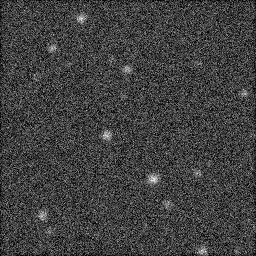
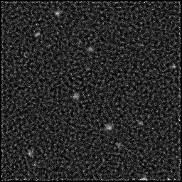
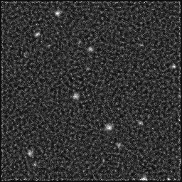
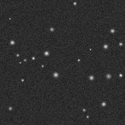
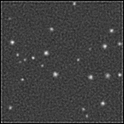
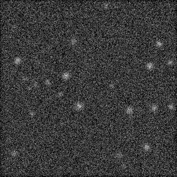
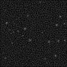
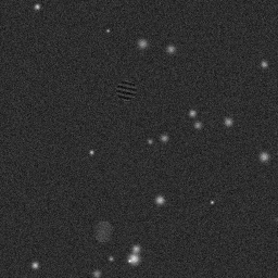
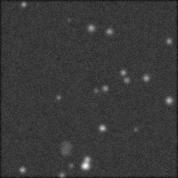
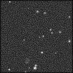
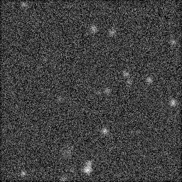
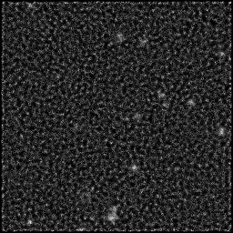
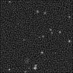
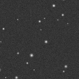
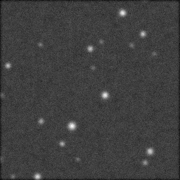
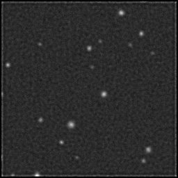
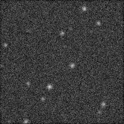
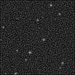
Reconstruction Gallery — 4 Scenes × 3 Scenarios
Method: CPU_baseline | Mismatch: nominal (nominal=True, perturbed=False)
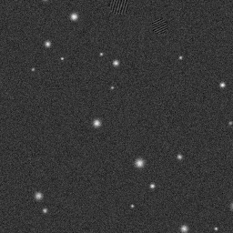
Ground Truth
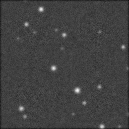
Measurement
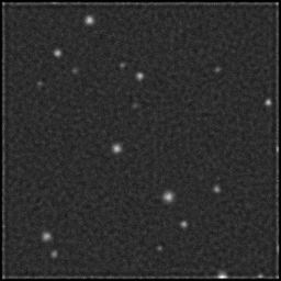
Reconstruction
Ground Truth
Measurement
Reconstruction
Ground Truth
Measurement (perturbed)
Reconstruction
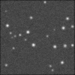
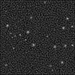
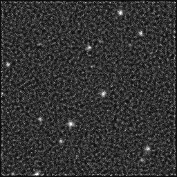
Mean PSNR Across All Scenes
Per-scene PSNR breakdown (4 scenes)
| Scene | I (PSNR) | I (SSIM) | II (PSNR) | II (SSIM) | III (PSNR) | III (SSIM) |
|---|---|---|---|---|---|---|
| scene_00 | 23.51322858456625 | 0.3680334261076263 | 18.321872109157592 | 0.10385815436617447 | 20.03444592103245 | 0.1989493017944018 |
| scene_01 | 20.039820761387634 | 0.29166542696823705 | 18.85922982415404 | 0.12798625129650684 | 20.031642094176974 | 0.19752602173448866 |
| scene_02 | 23.283012767044198 | 0.357495155445897 | 18.4465452279848 | 0.09369496983474383 | 20.2796683331393 | 0.18597290071365627 |
| scene_03 | 23.31589368033676 | 0.36687406178777526 | 18.405990402819242 | 0.10758808193384366 | 20.100674151892584 | 0.20008535528637864 |
| Mean | 22.53798894833371 | 0.3460170175773839 | 18.50840939102892 | 0.10828186435781721 | 20.111607625060326 | 0.19563339488223133 |
Experimental Setup
Key References
- Egerton, 'Electron Energy-Loss Spectroscopy in the Electron Microscope', Springer (2011)
Canonical Datasets
- EELS Atlas (Ahn & Krivanek)
Spec DAG — Forward Model Pipeline
P(e⁻) → Λ(energy) → D(g, η₁)
Mismatch Parameters
| Symbol | Parameter | Description | Nominal | Perturbed |
|---|---|---|---|---|
| ΔD_E | energy_dispersion | Energy dispersion error (eV/channel) | 0 | 0.002 |
| ΔE_0 | zero_loss_shift | Zero-loss peak shift (eV) | 0 | 0.3 |
| ΔC_c | aberration | Chromatic aberration error (%) | 0 | 2.0 |
Credits System
Spec Primitives Reference (11 primitives)
Free-space or medium propagation kernel (Fresnel, Rayleigh-Sommerfeld).
Spatial or spatio-temporal amplitude modulation (coded aperture, SLM pattern).
Geometric projection operator (Radon transform, fan-beam, cone-beam).
Sampling in the Fourier / k-space domain (MRI, ptychography).
Shift-invariant convolution with a point-spread function (PSF).
Summation along a physical dimension (spectral, temporal, angular).
Sensor readout with gain g and noise model η (Gaussian, Poisson, mixed).
Patterned illumination (block, Hadamard, random) applied to the scene.
Spectral dispersion element (prism, grating) with shift α and aperture a.
Sample or gantry rotation (CT, electron tomography).
Spectral filter or monochromator selecting a wavelength band.