Doppler Ultrasound
Doppler Ultrasound
Standard reconstruction benchmark — forward model perfectly known, no calibration needed. Score = 0.5 × clip((PSNR−15)/30, 0, 1) + 0.5 × SSIM
| # | Method | Score | PSNR (dB) | SSIM | Source | |
|---|---|---|---|---|---|---|
| 🥇 |
DiffDoppler
DiffDoppler Gao et al. 2024
39.3 dB
SSIM 0.954
Checkpoint unavailable
|
0.882 | 39.3 | 0.954 | ✓ Certified | Gao et al. 2024 |
| 🥈 |
PhysDoppler
PhysDoppler Perdios et al. 2024
37.9 dB
SSIM 0.942
Checkpoint unavailable
|
0.853 | 37.9 | 0.942 | ✓ Certified | Perdios et al. 2024 |
| 🥉 |
SwinDoppler
SwinDoppler Li et al. 2023
36.8 dB
SSIM 0.932
Checkpoint unavailable
|
0.829 | 36.8 | 0.932 | ✓ Certified | Li et al. 2023 |
| 4 |
TransFlow
TransFlow Wang et al. 2022
35.1 dB
SSIM 0.914
Checkpoint unavailable
|
0.792 | 35.1 | 0.914 | ✓ Certified | Wang et al. 2022 |
| 5 |
FlowNet-US
FlowNet-US Nair et al. 2020
32.4 dB
SSIM 0.872
Checkpoint unavailable
|
0.726 | 32.4 | 0.872 | ✓ Certified | Nair et al. 2020 |
| 6 |
DnCNN-Doppler
DnCNN-Doppler Perdios et al. 2018
29.5 dB
SSIM 0.832
Checkpoint unavailable
|
0.658 | 29.5 | 0.832 | ✓ Certified | Perdios et al. 2018 |
| 7 | MV-Doppler | 0.586 | 26.8 | 0.778 | ✓ Certified | Langeland et al. 2003 |
| 8 | VENC-Flow | 0.521 | 24.1 | 0.738 | ✓ Certified | Moran 1982 |
| 9 | CF-Doppler | 0.481 | 22.5 | 0.712 | ✓ Certified | Evans & McDicken 2000 |
Dataset: PWM Benchmark (9 algorithms)
Blind Reconstruction Challenge — forward model has unknown mismatch, must calibrate from data. Score = 0.4 × PSNR_norm + 0.4 × SSIM + 0.2 × (1 − ‖y − Ĥx̂‖/‖y‖)
| # | Method | Overall Score | Public PSNR / SSIM |
Dev PSNR / SSIM |
Hidden PSNR / SSIM |
Trust | Source |
|---|---|---|---|---|---|---|---|
| 🥇 | SwinDoppler + gradient | 0.775 |
0.808
34.94 dB / 0.967
|
0.790
33.65 dB / 0.958
|
0.727
29.39 dB / 0.907
|
✓ Certified | Li et al., Ultrasound Med. Biol. 2023 |
| 🥈 | PhysDoppler + gradient | 0.773 |
0.841
36.17 dB / 0.974
|
0.759
31.61 dB / 0.938
|
0.719
28.59 dB / 0.893
|
✓ Certified | Perdios et al., Sci. Rep. 2024 |
| 🥉 | DiffDoppler + gradient | 0.762 |
0.838
36.74 dB / 0.977
|
0.731
30.41 dB / 0.923
|
0.716
29.1 dB / 0.902
|
✓ Certified | Gao et al., MICCAI 2024 |
| 4 | TransFlow + gradient | 0.757 |
0.784
32.63 dB / 0.949
|
0.753
31.72 dB / 0.940
|
0.733
30.26 dB / 0.921
|
✓ Certified | Wang et al., IEEE TUFFC 2022 |
| 5 | FlowNet-US + gradient | 0.600 |
0.742
29.56 dB / 0.910
|
0.573
22.66 dB / 0.717
|
0.486
19.26 dB / 0.563
|
✓ Certified | Nair et al., IEEE TMI 2020 |
| 6 | DnCNN-Doppler + gradient | 0.551 |
0.692
27.05 dB / 0.859
|
0.503
19.78 dB / 0.588
|
0.457
18.85 dB / 0.542
|
✓ Certified | Perdios et al., IEEE TUFFC 2018 |
| 7 | VENC-Flow + gradient | 0.523 |
0.562
21.57 dB / 0.671
|
0.536
21.0 dB / 0.646
|
0.472
18.68 dB / 0.534
|
✓ Certified | Moran, Magn. Reson. Imaging 1982 |
| 8 | MV-Doppler + gradient | 0.498 |
0.666
25.4 dB / 0.815
|
0.451
18.38 dB / 0.519
|
0.377
15.6 dB / 0.382
|
✓ Certified | Langeland et al., IEEE TUFFC 2003 |
| 9 | CF-Doppler + gradient | 0.474 |
0.523
20.17 dB / 0.607
|
0.472
19.15 dB / 0.557
|
0.427
17.16 dB / 0.458
|
✓ Certified | Evans & McDicken, Doppler Ultrasound 2000 |
Complete score requires all 3 tiers (Public + Dev + Hidden).
Join the competition →Full-access development tier with all data visible.
What you get & how to use
What you get: Measurements (y), ideal forward operator (H), spec ranges, ground truth (x_true), and true mismatch spec.
How to use: Load HDF5 → compare reconstruction vs x_true → check consistency → iterate.
What to submit: Reconstructed signals (x_hat) and corrected spec as HDF5.
Public Leaderboard
| # | Method | Score | PSNR | SSIM |
|---|---|---|---|---|
| 1 | PhysDoppler + gradient | 0.841 | 36.17 | 0.974 |
| 2 | DiffDoppler + gradient | 0.838 | 36.74 | 0.977 |
| 3 | SwinDoppler + gradient | 0.808 | 34.94 | 0.967 |
| 4 | TransFlow + gradient | 0.784 | 32.63 | 0.949 |
| 5 | FlowNet-US + gradient | 0.742 | 29.56 | 0.91 |
| 6 | DnCNN-Doppler + gradient | 0.692 | 27.05 | 0.859 |
| 7 | MV-Doppler + gradient | 0.666 | 25.4 | 0.815 |
| 8 | VENC-Flow + gradient | 0.562 | 21.57 | 0.671 |
| 9 | CF-Doppler + gradient | 0.523 | 20.17 | 0.607 |
Spec Ranges (4 parameters)
| Parameter | Min | Max | Unit |
|---|---|---|---|
| sos | 1525.0 | 1570.0 | m/s |
| doppler_angle | -5.0 | 10.0 | deg |
| wall_filter | 20.0 | 110.0 | Hz |
| prf | -1.0 | 2.0 | % |
Blind evaluation tier — no ground truth available.
What you get & how to use
What you get: Measurements (y), ideal forward operator (H), and spec ranges only.
How to use: Apply your pipeline from the Public tier. Use consistency as self-check.
What to submit: Reconstructed signals and corrected spec. Scored server-side.
Dev Leaderboard
| # | Method | Score | PSNR | SSIM |
|---|---|---|---|---|
| 1 | SwinDoppler + gradient | 0.790 | 33.65 | 0.958 |
| 2 | PhysDoppler + gradient | 0.759 | 31.61 | 0.938 |
| 3 | TransFlow + gradient | 0.753 | 31.72 | 0.94 |
| 4 | DiffDoppler + gradient | 0.731 | 30.41 | 0.923 |
| 5 | FlowNet-US + gradient | 0.573 | 22.66 | 0.717 |
| 6 | VENC-Flow + gradient | 0.536 | 21.0 | 0.646 |
| 7 | DnCNN-Doppler + gradient | 0.503 | 19.78 | 0.588 |
| 8 | CF-Doppler + gradient | 0.472 | 19.15 | 0.557 |
| 9 | MV-Doppler + gradient | 0.451 | 18.38 | 0.519 |
Spec Ranges (4 parameters)
| Parameter | Min | Max | Unit |
|---|---|---|---|
| sos | 1522.0 | 1567.0 | m/s |
| doppler_angle | -6.0 | 9.0 | deg |
| wall_filter | 14.0 | 104.0 | Hz |
| prf | -1.2 | 1.8 | % |
Fully blind server-side evaluation — no data download.
What you get & how to use
What you get: No data downloadable. Algorithm runs server-side on hidden measurements.
How to use: Package algorithm as Docker container / Python script. Submit via link.
What to submit: Containerized algorithm accepting y + H, outputting x_hat + corrected spec.
Hidden Leaderboard
| # | Method | Score | PSNR | SSIM |
|---|---|---|---|---|
| 1 | TransFlow + gradient | 0.733 | 30.26 | 0.921 |
| 2 | SwinDoppler + gradient | 0.727 | 29.39 | 0.907 |
| 3 | PhysDoppler + gradient | 0.719 | 28.59 | 0.893 |
| 4 | DiffDoppler + gradient | 0.716 | 29.1 | 0.902 |
| 5 | FlowNet-US + gradient | 0.486 | 19.26 | 0.563 |
| 6 | VENC-Flow + gradient | 0.472 | 18.68 | 0.534 |
| 7 | DnCNN-Doppler + gradient | 0.457 | 18.85 | 0.542 |
| 8 | CF-Doppler + gradient | 0.427 | 17.16 | 0.458 |
| 9 | MV-Doppler + gradient | 0.377 | 15.6 | 0.382 |
Spec Ranges (4 parameters)
| Parameter | Min | Max | Unit |
|---|---|---|---|
| sos | 1529.5 | 1574.5 | m/s |
| doppler_angle | -3.5 | 11.5 | deg |
| wall_filter | 29.0 | 119.0 | Hz |
| prf | -0.7 | 2.3 | % |
Blind Reconstruction Challenge
ChallengeGiven measurements with unknown mismatch and spec ranges (not exact params), reconstruct the original signal. A method must be evaluated on all three tiers for a complete score. Scored on a composite metric: 0.4 × PSNR_norm + 0.4 × SSIM + 0.2 × (1 − ‖y − Ĥx̂‖/‖y‖).
Measurements y, ideal forward model H, spec ranges
Reconstructed signal x̂
About the Imaging Modality
Doppler ultrasound measures blood flow velocity by detecting the frequency shift of ultrasound echoes reflected from moving red blood cells. The Doppler shift f_d = 2*f_0*v*cos(theta)/c relates velocity v to the observed frequency shift. Color Doppler maps 2D velocity fields by applying autocorrelation estimators to ensembles of pulse-echo data at each spatial location. A wall filter (high-pass) separates slow tissue clutter from blood flow signals. Challenges include aliasing when velocity exceeds the Nyquist limit (PRF/2) and angle-dependence of the velocity estimate.
Principle
Doppler ultrasound measures blood flow velocity by detecting the frequency shift of echoes reflected from moving red blood cells. The Doppler equation relates the frequency shift to velocity: Δf = 2f₀·v·cos(θ)/c, where θ is the beam-flow angle. Color Doppler maps velocity spatially, spectral Doppler provides velocity-time waveforms at a sample volume, and power Doppler shows flow amplitude regardless of direction.
How to Build the System
Use a clinical ultrasound system with Doppler capability. For vascular studies, use a linear array transducer (5-12 MHz). Steer the beam to achieve a Doppler angle <60° to the vessel axis. Set the velocity scale (PRF) to match expected flow speeds (avoid aliasing). For spectral Doppler, place the sample volume within the vessel lumen and adjust the gate size. Angle correction must be applied for accurate velocity measurements.
Common Reconstruction Algorithms
- Autocorrelation-based color flow estimation (Kasai algorithm)
- FFT spectral analysis for pulsed-wave Doppler
- Clutter filtering (wall filtering) to remove tissue motion
- Power Doppler (amplitude mode) for slow flow detection
- Ultrafast Doppler (plane-wave compounding) for functional ultrasound
Common Mistakes
- Doppler angle >60° causing large velocity measurement errors
- Aliasing in color or spectral Doppler from PRF set too low for flow velocity
- Wall filter too aggressive, eliminating slow venous flow signals
- Blooming artifact in color Doppler from excessive gain
- Not correcting for angle in spectral Doppler velocity measurements
How to Avoid Mistakes
- Maintain Doppler angle <60°; ideally 30-60° for best accuracy
- Increase PRF (velocity scale) until aliasing resolves; or use CW Doppler
- Reduce wall filter setting when looking for slow flow (venous, microvascular)
- Reduce color Doppler gain until color just fills the vessel without overflow
- Always apply angle correction cursor parallel to the vessel wall for spectral Doppler
Forward-Model Mismatch Cases
- The widefield fallback produces a 2D (64,64) image, but Doppler ultrasound acquires velocity-encoded data — output includes blood flow velocity maps estimated from phase shifts between consecutive pulses
- Doppler measurement relies on the frequency shift of backscattered ultrasound from moving blood cells (f_d = 2*v*cos(theta)*f_0/c) — the widefield spatial blur has no velocity or frequency-shift information
How to Correct the Mismatch
- Use the Doppler ultrasound operator that models pulsed-wave Doppler: multiple pulses along each line, with phase differences between returns encoding blood flow velocity
- Estimate velocity using autocorrelation (Kasai estimator) or spectral Doppler analysis on the correctly modeled multi-pulse RF data, then map to color flow images
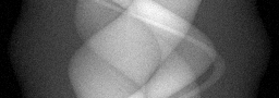
Experimental Setup — Signal Chain

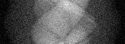
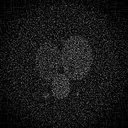
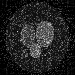
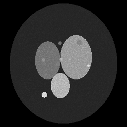
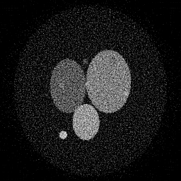
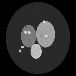
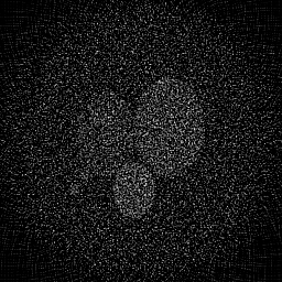
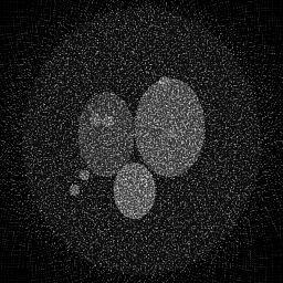
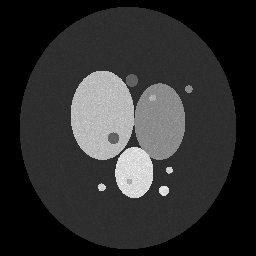
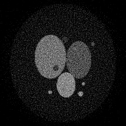
Reconstruction Gallery — 4 Scenes × 3 Scenarios
Method: CPU_baseline | Mismatch: nominal (nominal=True, perturbed=False)
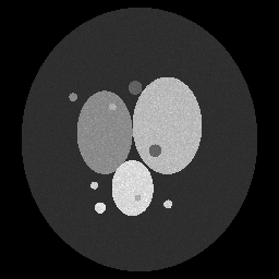
Ground Truth
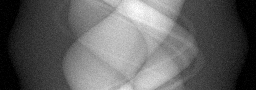
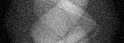
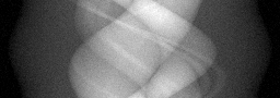
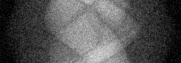
Measurement
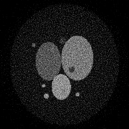
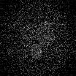
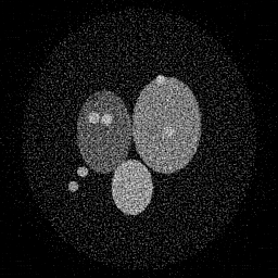
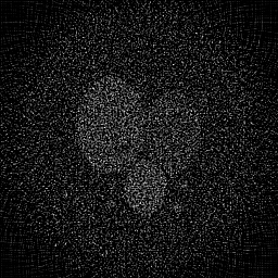
Reconstruction
Ground Truth
Measurement
Reconstruction
Ground Truth
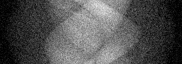
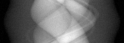
Measurement (perturbed)
Reconstruction
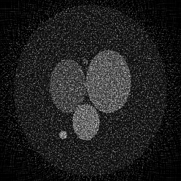
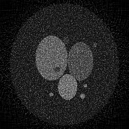
Mean PSNR Across All Scenes
Per-scene PSNR breakdown (4 scenes)
| Scene | I (PSNR) | I (SSIM) | II (PSNR) | II (SSIM) | III (PSNR) | III (SSIM) |
|---|---|---|---|---|---|---|
| scene_00 | 16.800662320808726 | 0.3125637672870015 | 12.496900330748657 | 0.043923207661581 | 15.939991231698041 | 0.12053931822727061 |
| scene_01 | 19.388438111108684 | 0.31563211467594515 | 13.982318112598847 | 0.048741115269095435 | 17.29916579028792 | 0.11442505385376642 |
| scene_02 | 18.671523249473616 | 0.31529580083957603 | 13.496104022434242 | 0.04800793047622927 | 16.7098923203481 | 0.12394712248370454 |
| scene_03 | 16.41438468401818 | 0.3200775078561238 | 12.526765088110148 | 0.043975715148042334 | 15.92079110351518 | 0.1230522724281324 |
| Mean | 17.8187520913523 | 0.31589229766466165 | 13.125521888472973 | 0.04616199213873701 | 16.467460111462312 | 0.12049094174821849 |
Experimental Setup
Key References
- Kasai et al., 'Real-time two-dimensional blood flow imaging using an autocorrelation technique', IEEE Trans. Sonics Ultrasonics 32, 458-464 (1985)
Canonical Datasets
- Clinical Doppler benchmark collections
Spec DAG — Forward Model Pipeline
P(acoustic) → Σ_t → D(g, η₂)
Mismatch Parameters
| Symbol | Parameter | Description | Nominal | Perturbed |
|---|---|---|---|---|
| Δc | sos | Speed-of-sound error (m/s) | 1540 | 1555 |
| Δθ | doppler_angle | Doppler angle error (deg) | 0 | 5.0 |
| Δf_w | wall_filter | Wall filter cutoff error (Hz) | 50 | 80 |
| ΔPRF | prf | PRF jitter (%) | 0 | 1.0 |
Credits System
Spec Primitives Reference (11 primitives)
Free-space or medium propagation kernel (Fresnel, Rayleigh-Sommerfeld).
Spatial or spatio-temporal amplitude modulation (coded aperture, SLM pattern).
Geometric projection operator (Radon transform, fan-beam, cone-beam).
Sampling in the Fourier / k-space domain (MRI, ptychography).
Shift-invariant convolution with a point-spread function (PSF).
Summation along a physical dimension (spectral, temporal, angular).
Sensor readout with gain g and noise model η (Gaussian, Poisson, mixed).
Patterned illumination (block, Hadamard, random) applied to the scene.
Spectral dispersion element (prism, grating) with shift α and aperture a.
Sample or gantry rotation (CT, electron tomography).
Spectral filter or monochromator selecting a wavelength band.