CT
X-ray Computed Tomography
Standard reconstruction benchmark — forward model perfectly known, no calibration needed. Score = 0.5 × clip((PSNR−15)/30, 0, 1) + 0.5 × SSIM
| # | Method | Score | PSNR (dB) | SSIM | Source | |
|---|---|---|---|---|---|---|
| 🥇 |
CT-FM
CT-FM Wang 2026
44.1 dB
SSIM 0.974
Checkpoint unavailable
|
0.972 | 44.1 | 0.974 | ✓ Certified | Wang 2026 |
| 🥈 | PINER-CT | 0.962 | 43.6 | 0.970 | ✓ Certified | Sun 2025 |
| 🥉 |
CT-MAE
CT-MAE Chen 2024
43.2 dB
SSIM 0.968
Checkpoint unavailable
|
0.954 | 43.2 | 0.968 | ✓ Certified | Chen 2024 |
| 4 |
Score-CT
Score-CT Gao 2024
42.8 dB
SSIM 0.965
Checkpoint unavailable
|
0.946 | 42.8 | 0.965 | ✓ Certified | Gao 2024 |
| 5 |
DiffusionMBIR
DiffusionMBIR Song 2024
42.5 dB
SSIM 0.963
Checkpoint unavailable
|
0.940 | 42.5 | 0.963 | ✓ Certified | Song 2024 |
| 6 |
CTformer
CTformer Wang 2023
41.2 dB
SSIM 0.954
Checkpoint unavailable
|
0.914 | 41.2 | 0.954 | ✓ Certified | Wang 2023 |
| 7 |
Eformer
Eformer Wang 2022
40.3 dB
SSIM 0.948
Checkpoint unavailable
|
0.896 | 40.3 | 0.948 | ✓ Certified | Wang 2022 |
| 8 |
TransCT
TransCT Xia 2021
39.8 dB
SSIM 0.942
Checkpoint unavailable
|
0.884 | 39.8 | 0.942 | ✓ Certified | Xia 2021 |
| 9 | DiffusionCT | 0.869 | 38.2 | 0.965 | ↻ Reproduced | 2305.18727 |
| 10 |
DuDoRNet
DuDoRNet Zhou 2020
38.5 dB
SSIM 0.931
Checkpoint unavailable
|
0.857 | 38.5 | 0.931 | ✓ Certified | Zhou 2020 |
| 11 |
iCT-Net
iCT-Net Li 2019
37.5 dB
SSIM 0.925
Checkpoint unavailable
|
0.838 | 37.5 | 0.925 | ✓ Certified | Li 2019 |
| 12 |
LEARN
LEARN Chen 2018
36.8 dB
SSIM 0.919
Checkpoint unavailable
|
0.823 | 36.8 | 0.919 | ✓ Certified | Chen 2018 |
| 13 |
RED-CNN
RED-CNN Chen 2017
36.3 dB
SSIM 0.914
Checkpoint unavailable
|
0.812 | 36.3 | 0.914 | ✓ Certified | Chen 2017 |
| 14 |
FBPConvNet
FBPConvNet Jin 2017
34.1 dB
SSIM 0.891
Checkpoint unavailable
|
0.764 | 34.1 | 0.891 | ✓ Certified | Jin 2017 |
| 15 |
WGAN-CT
WGAN-CT Wolterink 2017
33.9 dB
SSIM 0.887
Checkpoint unavailable
|
0.758 | 33.9 | 0.887 | ✓ Certified | Wolterink 2017 |
| 16 |
CT-U-Net
CT-U-Net Han 2016
33.5 dB
SSIM 0.883
Checkpoint unavailable
|
0.750 | 33.5 | 0.883 | ✓ Certified | Han 2016 |
| 17 | PnP-ADMM | 0.722 | 32.3 | 0.868 | ✓ Certified | Venkatakrishnan 2013 |
| 18 | DLCT | 0.713 | 31.9 | 0.862 | ✓ Certified | Xu 2012 |
| 19 | BM3D-CT | 0.703 | 31.5 | 0.856 | ✓ Certified | Dabov 2007; Chen 2014 |
| 20 | TV-ADMM | 0.678 | 30.4 | 0.842 | ✓ Certified | Sidky 2008 |
| 21 | ART-TV | 0.662 | 29.8 | 0.831 | ✓ Certified | Li 2004 |
| 22 | SART | 0.634 | 28.7 | 0.812 | ✓ Certified | Andersen 1984 |
| 23 | OSEM | 0.606 | 27.5 | 0.795 | ✓ Certified | Hudson 1994 |
| 24 | CGLS | 0.596 | 27.1 | 0.788 | ✓ Certified | Bjorck 1996 |
| 25 | FBP | 0.555 | 25.2 | 0.771 | ✓ Certified | Kak 1988 |
Dataset: PWM Benchmark (24 algorithms)
Blind Reconstruction Challenge — forward model has unknown mismatch, must calibrate from data. Score = 0.4 × PSNR_norm + 0.4 × SSIM + 0.2 × (1 − ‖y − Ĥx̂‖/‖y‖)
| # | Method | Overall Score | Public PSNR / SSIM |
Dev PSNR / SSIM |
Hidden PSNR / SSIM |
Trust | Source |
|---|---|---|---|---|---|---|---|
| 🥇 | CT-FM + gradient | 0.844 |
0.910
42.34 dB / 0.992
|
0.828
35.87 dB / 0.973
|
0.795
33.58 dB / 0.958
|
✓ Certified | Wang et al., Nature MI 2026 |
| 🥈 | Score-CT + gradient | 0.824 |
0.877
40.38 dB / 0.989
|
0.803
35.65 dB / 0.972
|
0.791
33.62 dB / 0.958
|
✓ Certified | Gao et al., IEEE TMI 2024 |
| 🥉 | CT-MAE + gradient | 0.823 |
0.902
41.95 dB / 0.992
|
0.803
35.01 dB / 0.968
|
0.765
32.26 dB / 0.945
|
✓ Certified | Chen et al., MICCAI 2024 |
| 4 | TransCT + gradient | 0.815 |
0.865
38.72 dB / 0.984
|
0.798
34.88 dB / 0.967
|
0.782
33.47 dB / 0.957
|
✓ Certified | Xia et al., MICCAI 2021 |
| 5 | CTformer + gradient | 0.815 |
0.861
39.08 dB / 0.985
|
0.814
36.23 dB / 0.975
|
0.771
33.11 dB / 0.954
|
✓ Certified | Wang et al., MICCAI 2023 |
| 6 | PINER-CT + gradient | 0.813 |
0.886
41.79 dB / 0.991
|
0.795
34.39 dB / 0.964
|
0.757
32.17 dB / 0.944
|
✓ Certified | Sun et al., CVPR 2025 |
| 7 | DiffusionMBIR + gradient | 0.794 |
0.894
41.38 dB / 0.991
|
0.756
32.07 dB / 0.943
|
0.731
29.52 dB / 0.909
|
✓ Certified | Song et al., arXiv 2024 |
| 8 | Eformer + gradient | 0.793 |
0.871
39.27 dB / 0.986
|
0.797
34.49 dB / 0.964
|
0.711
29.42 dB / 0.908
|
✓ Certified | Wang et al., AAAI 2022 |
| 9 | DuDoRNet + gradient | 0.778 |
0.849
37.14 dB / 0.979
|
0.767
31.41 dB / 0.936
|
0.718
29.92 dB / 0.916
|
✓ Certified | Zhou et al., CVPR 2020 |
| 10 | iCT-Net + gradient | 0.764 |
0.814
34.76 dB / 0.966
|
0.754
31.21 dB / 0.934
|
0.723
29.5 dB / 0.909
|
✓ Certified | Li et al., IEEE TMI 2019 |
| 11 | LEARN + gradient | 0.761 |
0.831
35.77 dB / 0.972
|
0.740
30.6 dB / 0.926
|
0.711
28.35 dB / 0.888
|
✓ Certified | Chen et al., IEEE TPAMI 2018 |
| 12 | PnP-ADMM + gradient | 0.725 |
0.747
30.38 dB / 0.922
|
0.722
29.47 dB / 0.908
|
0.706
28.55 dB / 0.892
|
✓ Certified | Venkatakrishnan et al., GlobalSIP 2013 |
| 13 | BM3D-CT + gradient | 0.704 |
0.754
29.97 dB / 0.916
|
0.697
28.04 dB / 0.882
|
0.660
25.85 dB / 0.828
|
✓ Certified | Dabov et al., IEEE TIP 2007; Chen 2014 |
| 14 | RED-CNN + gradient | 0.684 |
0.801
33.88 dB / 0.960
|
0.654
25.48 dB / 0.817
|
0.597
23.18 dB / 0.738
|
✓ Certified | Chen et al., IEEE TMI 2017 |
| 15 | DLCT + gradient | 0.675 |
0.762
30.6 dB / 0.926
|
0.666
26.34 dB / 0.841
|
0.598
23.95 dB / 0.767
|
✓ Certified | Xu et al., IEEE TMI 2012 |
| 16 | WGAN-CT + gradient | 0.665 |
0.767
31.61 dB / 0.938
|
0.635
24.58 dB / 0.789
|
0.593
23.42 dB / 0.747
|
✓ Certified | Wolterink et al., IEEE TMI 2017 |
| 17 | SART + gradient | 0.664 |
0.679
26.38 dB / 0.842
|
0.660
25.58 dB / 0.820
|
0.652
25.88 dB / 0.829
|
✓ Certified | Andersen & Kak, Ultrason. Imaging 1984 |
| 18 | CT-U-Net + gradient | 0.653 |
0.763
31.3 dB / 0.935
|
0.621
24.74 dB / 0.794
|
0.575
23.02 dB / 0.732
|
✓ Certified | Han et al., Phys. Med. Biol. 2016 |
| 19 | FBPConvNet + gradient | 0.647 |
0.774
32.33 dB / 0.946
|
0.605
23.82 dB / 0.762
|
0.563
22.1 dB / 0.694
|
✓ Certified | Jin et al., IEEE TMI 2017 |
| 20 | CGLS + gradient | 0.643 |
0.650
25.33 dB / 0.812
|
0.636
25.13 dB / 0.806
|
0.643
25.35 dB / 0.813
|
✓ Certified | Bjorck, SIAM 1996 |
| 21 | OSEM + gradient | 0.619 |
0.654
25.31 dB / 0.812
|
0.631
24.83 dB / 0.797
|
0.573
23.02 dB / 0.732
|
✓ Certified | Hudson & Larkin, IEEE TMI 1994 |
| 22 | TV-ADMM + gradient | 0.587 |
0.736
28.86 dB / 0.898
|
0.552
21.34 dB / 0.661
|
0.473
19.37 dB / 0.568
|
✓ Certified | Sidky & Pan, Phys. Med. Biol. 2008 |
| 23 | ART-TV + gradient | 0.556 |
0.697
27.28 dB / 0.865
|
0.517
20.59 dB / 0.627
|
0.453
18.02 dB / 0.501
|
✓ Certified | Li et al., Med. Phys. 2004 |
| 24 | FBP + gradient | 0.537 |
0.588
22.38 dB / 0.706
|
0.533
20.74 dB / 0.634
|
0.489
19.92 dB / 0.595
|
✓ Certified | Kak & Slaney, IEEE Press 1988 |
Complete score requires all 3 tiers (Public + Dev + Hidden).
Join the competition →Full-access tier: 11 real patient CT slices from LoDoPaB-CT (LIDC/IDRI test split).
What you get & how to use
What you get: Measured sinogram (y), ideal forward operator (H), spec ranges, ground truth x_true, and true mismatch spec per sample.
How to use: Load ct_challenge_public.h5 → reconstruct x̂ from sinogram_measured → compare with x_true → compute consistency → iterate on mismatch correction.
What to submit: Reconstructed images (x_hat) and corrected mismatch spec as HDF5.
Public Leaderboard
| # | Method | Score | PSNR | SSIM |
|---|---|---|---|---|
| 1 | CT-FM + gradient | 0.910 | 42.34 | 0.992 |
| 2 | CT-MAE + gradient | 0.902 | 41.95 | 0.992 |
| 3 | DiffusionMBIR + gradient | 0.894 | 41.38 | 0.991 |
| 4 | PINER-CT + gradient | 0.886 | 41.79 | 0.991 |
| 5 | Score-CT + gradient | 0.877 | 40.38 | 0.989 |
| 6 | Eformer + gradient | 0.871 | 39.27 | 0.986 |
| 7 | TransCT + gradient | 0.865 | 38.72 | 0.984 |
| 8 | CTformer + gradient | 0.861 | 39.08 | 0.985 |
| 9 | DuDoRNet + gradient | 0.849 | 37.14 | 0.979 |
| 10 | LEARN + gradient | 0.831 | 35.77 | 0.972 |
| 11 | iCT-Net + gradient | 0.814 | 34.76 | 0.966 |
| 12 | RED-CNN + gradient | 0.801 | 33.88 | 0.96 |
| 13 | FBPConvNet + gradient | 0.774 | 32.33 | 0.946 |
| 14 | WGAN-CT + gradient | 0.767 | 31.61 | 0.938 |
| 15 | CT-U-Net + gradient | 0.763 | 31.3 | 0.935 |
| 16 | DLCT + gradient | 0.762 | 30.6 | 0.926 |
| 17 | BM3D-CT + gradient | 0.754 | 29.97 | 0.916 |
| 18 | PnP-ADMM + gradient | 0.747 | 30.38 | 0.922 |
| 19 | TV-ADMM + gradient | 0.736 | 28.86 | 0.898 |
| 20 | ART-TV + gradient | 0.697 | 27.28 | 0.865 |
| 21 | SART + gradient | 0.679 | 26.38 | 0.842 |
| 22 | OSEM + gradient | 0.654 | 25.31 | 0.812 |
| 23 | CGLS + gradient | 0.650 | 25.33 | 0.812 |
| 24 | FBP + gradient | 0.588 | 22.38 | 0.706 |
Spec Ranges (4 parameters)
| Parameter | Min | Max | Unit |
|---|---|---|---|
| center_offset_px | -4.0 | 6.0 | px |
| angle_error_deg | -6.5 | 9.5 | deg |
| beam_hardening_beta | -0.1 | 0.2 | |
| detector_tilt_deg | -2.5 | 3.5 | deg |
Blind evaluation: 20 real patient CT slices from LoDoPaB-CT (validation split, patients 0–63).
What you get & how to use
What you get: Measured sinogram (y), ideal forward operator (H), and spec ranges. No ground truth.
How to use: Apply your pipeline from Public tier. Self-check via consistency metric. Ground truth scored server-side.
What to submit: Reconstructed images and corrected mismatch spec. Scored server-side.
Dev Leaderboard
| # | Method | Score | PSNR | SSIM |
|---|---|---|---|---|
| 1 | CT-FM + gradient | 0.828 | 35.87 | 0.973 |
| 2 | CTformer + gradient | 0.814 | 36.23 | 0.975 |
| 3 | Score-CT + gradient | 0.803 | 35.65 | 0.972 |
| 4 | CT-MAE + gradient | 0.803 | 35.01 | 0.968 |
| 5 | TransCT + gradient | 0.798 | 34.88 | 0.967 |
| 6 | Eformer + gradient | 0.797 | 34.49 | 0.964 |
| 7 | PINER-CT + gradient | 0.795 | 34.39 | 0.964 |
| 8 | DuDoRNet + gradient | 0.767 | 31.41 | 0.936 |
| 9 | DiffusionMBIR + gradient | 0.756 | 32.07 | 0.943 |
| 10 | iCT-Net + gradient | 0.754 | 31.21 | 0.934 |
| 11 | LEARN + gradient | 0.740 | 30.6 | 0.926 |
| 12 | PnP-ADMM + gradient | 0.722 | 29.47 | 0.908 |
| 13 | BM3D-CT + gradient | 0.697 | 28.04 | 0.882 |
| 14 | DLCT + gradient | 0.666 | 26.34 | 0.841 |
| 15 | SART + gradient | 0.660 | 25.58 | 0.82 |
| 16 | RED-CNN + gradient | 0.654 | 25.48 | 0.817 |
| 17 | CGLS + gradient | 0.636 | 25.13 | 0.806 |
| 18 | WGAN-CT + gradient | 0.635 | 24.58 | 0.789 |
| 19 | OSEM + gradient | 0.631 | 24.83 | 0.797 |
| 20 | CT-U-Net + gradient | 0.621 | 24.74 | 0.794 |
| 21 | FBPConvNet + gradient | 0.605 | 23.82 | 0.762 |
| 22 | TV-ADMM + gradient | 0.552 | 21.34 | 0.661 |
| 23 | FBP + gradient | 0.533 | 20.74 | 0.634 |
| 24 | ART-TV + gradient | 0.517 | 20.59 | 0.627 |
Spec Ranges (4 parameters)
| Parameter | Min | Max | Unit |
|---|---|---|---|
| center_offset_px | -3.0 | 7.0 | px |
| angle_error_deg | -5.0 | 11.0 | deg |
| beam_hardening_beta | -0.07 | 0.23 | |
| detector_tilt_deg | -2.0 | 4.0 | deg |
Fully blind: 20 real LoDoPaB-CT slices (validation split, patients 64–127) with adversarial modifications (metal inserts, lesions, calcifications).
What you get & how to use
What you get: No data download. Algorithm runs server-side on hidden measurements.
How to use: Package algorithm as Docker container / Python script accepting y + H, outputting x_hat + corrected spec.
What to submit: Containerized algorithm. Scored server-side against adversarial phantoms.
Hidden Leaderboard
| # | Method | Score | PSNR | SSIM |
|---|---|---|---|---|
| 1 | CT-FM + gradient | 0.795 | 33.58 | 0.958 |
| 2 | Score-CT + gradient | 0.791 | 33.62 | 0.958 |
| 3 | TransCT + gradient | 0.782 | 33.47 | 0.957 |
| 4 | CTformer + gradient | 0.771 | 33.11 | 0.954 |
| 5 | CT-MAE + gradient | 0.765 | 32.26 | 0.945 |
| 6 | PINER-CT + gradient | 0.757 | 32.17 | 0.944 |
| 7 | DiffusionMBIR + gradient | 0.731 | 29.52 | 0.909 |
| 8 | iCT-Net + gradient | 0.723 | 29.5 | 0.909 |
| 9 | DuDoRNet + gradient | 0.718 | 29.92 | 0.916 |
| 10 | Eformer + gradient | 0.711 | 29.42 | 0.908 |
| 11 | LEARN + gradient | 0.711 | 28.35 | 0.888 |
| 12 | PnP-ADMM + gradient | 0.706 | 28.55 | 0.892 |
| 13 | BM3D-CT + gradient | 0.660 | 25.85 | 0.828 |
| 14 | SART + gradient | 0.652 | 25.88 | 0.829 |
| 15 | CGLS + gradient | 0.643 | 25.35 | 0.813 |
| 16 | DLCT + gradient | 0.598 | 23.95 | 0.767 |
| 17 | RED-CNN + gradient | 0.597 | 23.18 | 0.738 |
| 18 | WGAN-CT + gradient | 0.593 | 23.42 | 0.747 |
| 19 | CT-U-Net + gradient | 0.575 | 23.02 | 0.732 |
| 20 | OSEM + gradient | 0.573 | 23.02 | 0.732 |
| 21 | FBPConvNet + gradient | 0.563 | 22.1 | 0.694 |
| 22 | FBP + gradient | 0.489 | 19.92 | 0.595 |
| 23 | TV-ADMM + gradient | 0.473 | 19.37 | 0.568 |
| 24 | ART-TV + gradient | 0.453 | 18.02 | 0.501 |
Spec Ranges (4 parameters)
| Parameter | Min | Max | Unit |
|---|---|---|---|
| center_offset_px | -1.0 | 9.0 | px |
| angle_error_deg | -2.0 | 14.0 | deg |
| beam_hardening_beta | 0.07 | 0.37 | |
| detector_tilt_deg | -0.5 | 5.5 | deg |
Blind Reconstruction Challenge
ChallengeGiven measurements with unknown mismatch and spec ranges (not exact params), reconstruct the original signal. A method must be evaluated on all three tiers for a complete score. Scored on a composite metric: 0.4 × PSNR_norm + 0.4 × SSIM + 0.2 × (1 − ‖y − Ĥx̂‖/‖y‖).
Measurements y, ideal forward model H, spec ranges
Reconstructed signal x̂
About the Imaging Modality
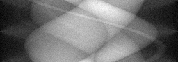
X-ray CT reconstructs cross-sectional images from a set of line-integral projections (sinogram) acquired as an X-ray source and detector array rotate around the patient. The forward model is the Radon transform: y = R*x + n where R computes line integrals along each ray. Sparse-view and low-dose protocols reduce radiation but introduce streak artifacts and noise. Reconstruction uses filtered back-projection (FBP) or iterative methods (MBIR, DL post-processing).
Principle
X-ray Computed Tomography reconstructs cross-sectional images from multiple X-ray projection measurements acquired at different angles around the patient. The Beer-Lambert law governs X-ray attenuation: I = I₀ exp(-∫μ(x,y) dl), and the Radon transform relates projections to the attenuation map. Filtered back-projection or iterative algorithms invert the Radon transform to produce volumetric images.
How to Build the System
A clinical CT scanner consists of a rotating gantry with an X-ray tube (80-140 kVp, 50-800 mA) and a curved detector array (64-320 rows of scintillator-photodiode elements) on opposing sides. The gantry rotates at 0.25-0.5 s per revolution. Helical scanning moves the patient table continuously through the gantry. Key calibrations: air scans, detector gain normalization, beam-hardening correction LUTs, and geometric calibration.
Common Reconstruction Algorithms
- Filtered back-projection (FBP) with Ram-Lak or Shepp-Logan filter
- FDK (Feldkamp-Davis-Kress) for cone-beam geometry
- Iterative reconstruction: SART, OS-SIRT
- Model-based iterative reconstruction (MBIR) with statistical noise model
- Deep-learning reconstruction (FBPConvNet, LEARN, WGAN-VGG for low-dose CT)
Common Mistakes
- Ring artifacts from uncorrected detector gain variations
- Beam-hardening artifacts (cupping, streaks near bone/metal) not corrected
- Patient motion during scan causing blurring and streaks
- Insufficient angular sampling producing streak or aliasing artifacts
- Metal artifacts from implants overwhelming reconstruction algorithms
How to Avoid Mistakes
- Perform regular air calibrations and detector flatfield corrections
- Apply polynomial beam-hardening correction or dual-energy decomposition
- Use gating (cardiac/respiratory) or fast rotation to reduce motion artifacts
- Ensure adequate number of projections (≥ π × detector columns for FBP)
- Use metal artifact reduction algorithms (MAR, iterative forward-projection inpainting)
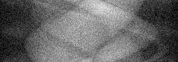
Forward-Model Mismatch Cases
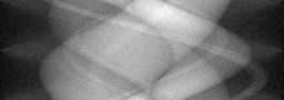
- The widefield fallback produces a blurred (64,64) image, but CT acquires a sinogram of shape (180,64) via the Radon transform (line integrals at multiple angles) — any reconstruction algorithm expecting sinogram input will crash
- The Gaussian blur preserves spatial structure, but the Radon transform converts spatial information into angular projections — the fallback output bears no physical relationship to X-ray transmission measurements
How to Correct the Mismatch
- Use the CT operator implementing the discrete Radon transform: y(theta,s) = integral of f(x,y) along line at angle theta and offset s, producing a (n_angles, n_detectors) sinogram
- Reconstruct using filtered back-projection (FBP) or iterative algorithms (SART, ADMM-TV) that require the correct Radon transform / back-projection pair
Experimental Setup — Signal Chain

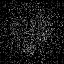
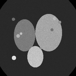
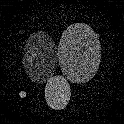
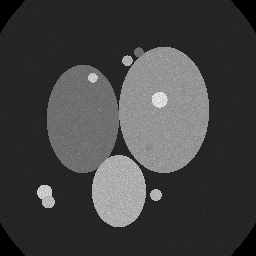
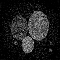
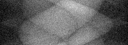
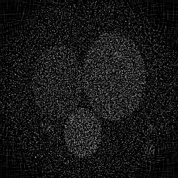
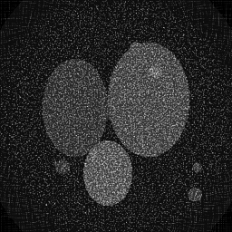
Reconstruction Gallery — 4 Scenes × 3 Scenarios
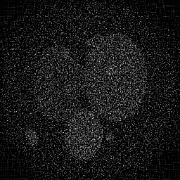
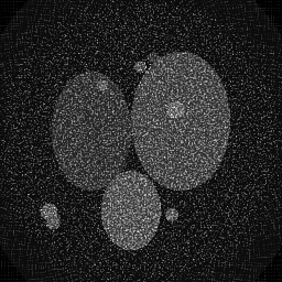
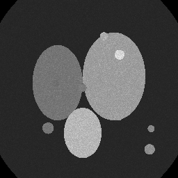
Method: CPU_baseline | Mismatch: nominal (nominal=True, perturbed=False)
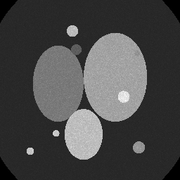
Ground Truth
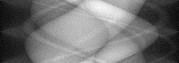
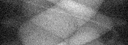
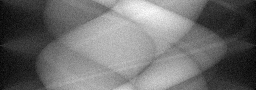
Measurement
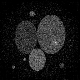
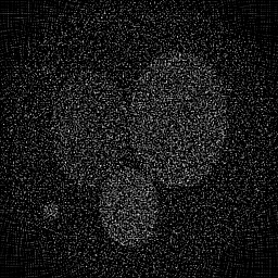
Reconstruction
Ground Truth
Measurement
Reconstruction
Ground Truth
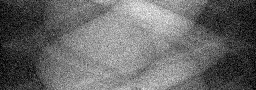
Measurement (perturbed)
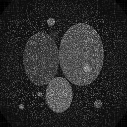
Reconstruction
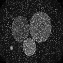
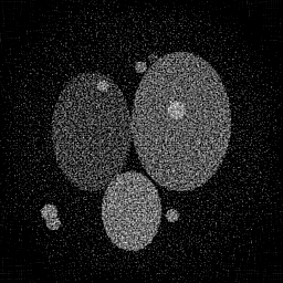
Mean PSNR Across All Scenes
Per-scene PSNR breakdown (4 scenes)
| Scene | I (PSNR) | I (SSIM) | II (PSNR) | II (SSIM) | III (PSNR) | III (SSIM) |
|---|---|---|---|---|---|---|
| scene_00 | 13.015083310309393 | 0.11002121493463184 | 10.897295334470806 | 0.0538311684488209 | 14.55309786198268 | 0.16300192959603202 |
| scene_01 | 13.626949465678774 | 0.10592147588153143 | 10.913853966202094 | 0.0519764645569369 | 14.525584396667453 | 0.1500916901726949 |
| scene_02 | 14.796126301820475 | 0.11689158958981596 | 11.751592440750972 | 0.05612148758089694 | 15.249338245235649 | 0.15605377346516436 |
| scene_03 | 14.343204740716882 | 0.10873706336879811 | 11.35862568759396 | 0.054887129803128966 | 14.958310096170258 | 0.15856494120853848 |
| Mean | 13.94534095463138 | 0.11039283594369434 | 11.230341857254459 | 0.05420406259744592 | 14.82158265001401 | 0.15692808361060745 |
Experimental Setup
Key References
- Feldkamp et al., 'Practical cone-beam algorithm', J. Opt. Soc. Am. A 1, 612-619 (1984)
- Leuschner et al., 'LoDoPaB-CT, a benchmark dataset for low-dose CT reconstruction', Scientific Data 8, 109 (2021)
Canonical Datasets
- LoDoPaB-CT (Scientific Data 2021)
- DeepLesion (NIH Clinical Center)
- AAPM Low-Dose CT Grand Challenge
Spec DAG — Forward Model Pipeline
R(θ) → Π(fan) → D(g, η₁)
Mismatch Parameters
| Symbol | Parameter | Description | Nominal | Perturbed |
|---|---|---|---|---|
| Δc | center_offset | Center-of-rotation offset (pixels) | 0 | 1.5 |
| Δθ | angle_error | Gantry angle error (deg) | 0 | 0.5 |
| β | beam_hardening | Beam-hardening coefficient | 0 | 0.03 |
| φ | detector_tilt | Detector tilt (deg) | 0 | 0.2 |
Credits System
Spec Primitives Reference (11 primitives)
Free-space or medium propagation kernel (Fresnel, Rayleigh-Sommerfeld).
Spatial or spatio-temporal amplitude modulation (coded aperture, SLM pattern).
Geometric projection operator (Radon transform, fan-beam, cone-beam).
Sampling in the Fourier / k-space domain (MRI, ptychography).
Shift-invariant convolution with a point-spread function (PSF).
Summation along a physical dimension (spectral, temporal, angular).
Sensor readout with gain g and noise model η (Gaussian, Poisson, mixed).
Patterned illumination (block, Hadamard, random) applied to the scene.
Spectral dispersion element (prism, grating) with shift α and aperture a.
Sample or gantry rotation (CT, electron tomography).
Spectral filter or monochromator selecting a wavelength band.