Confocal Live-Cell
Confocal Live-Cell Microscopy
Standard reconstruction benchmark — forward model perfectly known, no calibration needed. Score = 0.5 × clip((PSNR−15)/30, 0, 1) + 0.5 × SSIM
| # | Method | Score | PSNR (dB) | SSIM | Source | |
|---|---|---|---|---|---|---|
| 🥇 |
DiffusionCell
DiffusionCell Gao 2024
39.2 dB
SSIM 0.959
Checkpoint unavailable
|
0.883 | 39.2 | 0.959 | ✓ Certified | Gao 2024 |
| 🥈 |
Restormer-Micro
Restormer-Micro Zamir 2022
37.8 dB
SSIM 0.946
Checkpoint unavailable
|
0.853 | 37.8 | 0.946 | ✓ Certified | Zamir 2022 |
| 🥉 |
SwinIR-LiveCell
SwinIR-LiveCell Liang 2021
36.2 dB
SSIM 0.931
Checkpoint unavailable
|
0.819 | 36.2 | 0.931 | ✓ Certified | Liang 2021 |
| 4 |
CARE
CARE Weigert 2018
33.5 dB
SSIM 0.891
Checkpoint unavailable
|
0.754 | 33.5 | 0.891 | ✓ Certified | Weigert 2018 |
| 5 |
PN2V
PN2V Krull 2020
32.9 dB
SSIM 0.882
Checkpoint unavailable
|
0.739 | 32.9 | 0.882 | ✓ Certified | Krull 2020 |
| 6 |
Noise2Void
Noise2Void Krull 2019
31.8 dB
SSIM 0.871
Checkpoint unavailable
|
0.716 | 31.8 | 0.871 | ✓ Certified | Krull 2019 |
| 7 |
Noise2Self
Noise2Self Batson 2019
30.5 dB
SSIM 0.858
Checkpoint unavailable
|
0.687 | 30.5 | 0.858 | ✓ Certified | Batson 2019 |
| 8 | NLM-Fluorescence | 0.594 | 26.8 | 0.795 | ✓ Certified | Buades 2005 |
| 9 | VST-Denoise | 0.529 | 24.2 | 0.751 | ✓ Certified | Anscombe 1948 |
Dataset: PWM Benchmark (9 algorithms)
Blind Reconstruction Challenge — forward model has unknown mismatch, must calibrate from data. Score = 0.4 × PSNR_norm + 0.4 × SSIM + 0.2 × (1 − ‖y − Ĥx̂‖/‖y‖)
| # | Method | Overall Score | Public PSNR / SSIM |
Dev PSNR / SSIM |
Hidden PSNR / SSIM |
Trust | Source |
|---|---|---|---|---|---|---|---|
| 🥇 | DiffusionCell + gradient | 0.765 |
0.857
37.54 dB / 0.980
|
0.745
31.2 dB / 0.933
|
0.694
28.42 dB / 0.889
|
✓ Certified | Gao et al., Nat. Methods 2024 |
| 🥈 | Restormer-Micro + gradient | 0.758 |
0.841
36.47 dB / 0.976
|
0.755
31.19 dB / 0.933
|
0.678
26.52 dB / 0.846
|
✓ Certified | Zamir et al., CVPR 2022 (microscopy) |
| 🥉 | SwinIR-LiveCell + gradient | 0.742 |
0.824
35.19 dB / 0.969
|
0.733
30.13 dB / 0.919
|
0.669
26.67 dB / 0.850
|
✓ Certified | Liang et al., ICCV 2021 (live-cell) |
| 4 | PN2V + gradient | 0.655 |
0.775
31.29 dB / 0.935
|
0.616
23.69 dB / 0.757
|
0.574
22.67 dB / 0.718
|
✓ Certified | Krull et al., ECCV 2020 |
| 5 | Noise2Void + gradient | 0.639 |
0.738
29.81 dB / 0.914
|
0.605
24.05 dB / 0.770
|
0.575
22.26 dB / 0.701
|
✓ Certified | Krull et al., CVPR 2019 |
| 6 | CARE + gradient | 0.633 |
0.759
30.62 dB / 0.926
|
0.592
22.89 dB / 0.727
|
0.547
21.55 dB / 0.670
|
✓ Certified | Weigert et al., Nat. Methods 2018 |
| 7 | NLM-Fluorescence + gradient | 0.583 |
0.640
24.8 dB / 0.796
|
0.564
21.85 dB / 0.684
|
0.545
21.02 dB / 0.647
|
✓ Certified | Buades et al., CVPR 2005 |
| 8 | Noise2Self + gradient | 0.573 |
0.707
27.61 dB / 0.872
|
0.527
21.09 dB / 0.650
|
0.486
19.4 dB / 0.570
|
✓ Certified | Batson & Royer, ICML 2019 |
| 9 | VST-Denoise + gradient | 0.534 |
0.603
22.71 dB / 0.720
|
0.520
20.16 dB / 0.606
|
0.478
19.34 dB / 0.567
|
✓ Certified | Anscombe, Biometrika 1948 |
Complete score requires all 3 tiers (Public + Dev + Hidden).
Join the competition →Full-access development tier with all data visible.
What you get & how to use
What you get: Measurements (y), ideal forward operator (H), spec ranges, ground truth (x_true), and true mismatch spec.
How to use: Load HDF5 → compare reconstruction vs x_true → check consistency → iterate.
What to submit: Reconstructed signals (x_hat) and corrected spec as HDF5.
Public Leaderboard
| # | Method | Score | PSNR | SSIM |
|---|---|---|---|---|
| 1 | DiffusionCell + gradient | 0.857 | 37.54 | 0.98 |
| 2 | Restormer-Micro + gradient | 0.841 | 36.47 | 0.976 |
| 3 | SwinIR-LiveCell + gradient | 0.824 | 35.19 | 0.969 |
| 4 | PN2V + gradient | 0.775 | 31.29 | 0.935 |
| 5 | CARE + gradient | 0.759 | 30.62 | 0.926 |
| 6 | Noise2Void + gradient | 0.738 | 29.81 | 0.914 |
| 7 | Noise2Self + gradient | 0.707 | 27.61 | 0.872 |
| 8 | NLM-Fluorescence + gradient | 0.640 | 24.8 | 0.796 |
| 9 | VST-Denoise + gradient | 0.603 | 22.71 | 0.72 |
Spec Ranges (3 parameters)
| Parameter | Min | Max | Unit |
|---|---|---|---|
| pinhole | -5.0 | 10.0 | μm |
| refractive_index | 1.51 | 1.525 | |
| photobleaching | -5.0 | 10.0 | % |
Blind evaluation tier — no ground truth available.
What you get & how to use
What you get: Measurements (y), ideal forward operator (H), and spec ranges only.
How to use: Apply your pipeline from the Public tier. Use consistency as self-check.
What to submit: Reconstructed signals and corrected spec. Scored server-side.
Dev Leaderboard
| # | Method | Score | PSNR | SSIM |
|---|---|---|---|---|
| 1 | Restormer-Micro + gradient | 0.755 | 31.19 | 0.933 |
| 2 | DiffusionCell + gradient | 0.745 | 31.2 | 0.933 |
| 3 | SwinIR-LiveCell + gradient | 0.733 | 30.13 | 0.919 |
| 4 | PN2V + gradient | 0.616 | 23.69 | 0.757 |
| 5 | Noise2Void + gradient | 0.605 | 24.05 | 0.77 |
| 6 | CARE + gradient | 0.592 | 22.89 | 0.727 |
| 7 | NLM-Fluorescence + gradient | 0.564 | 21.85 | 0.684 |
| 8 | Noise2Self + gradient | 0.527 | 21.09 | 0.65 |
| 9 | VST-Denoise + gradient | 0.520 | 20.16 | 0.606 |
Spec Ranges (3 parameters)
| Parameter | Min | Max | Unit |
|---|---|---|---|
| pinhole | -6.0 | 9.0 | μm |
| refractive_index | 1.509 | 1.524 | |
| photobleaching | -6.0 | 9.0 | % |
Fully blind server-side evaluation — no data download.
What you get & how to use
What you get: No data downloadable. Algorithm runs server-side on hidden measurements.
How to use: Package algorithm as Docker container / Python script. Submit via link.
What to submit: Containerized algorithm accepting y + H, outputting x_hat + corrected spec.
Hidden Leaderboard
| # | Method | Score | PSNR | SSIM |
|---|---|---|---|---|
| 1 | DiffusionCell + gradient | 0.694 | 28.42 | 0.889 |
| 2 | Restormer-Micro + gradient | 0.678 | 26.52 | 0.846 |
| 3 | SwinIR-LiveCell + gradient | 0.669 | 26.67 | 0.85 |
| 4 | Noise2Void + gradient | 0.575 | 22.26 | 0.701 |
| 5 | PN2V + gradient | 0.574 | 22.67 | 0.718 |
| 6 | CARE + gradient | 0.547 | 21.55 | 0.67 |
| 7 | NLM-Fluorescence + gradient | 0.545 | 21.02 | 0.647 |
| 8 | Noise2Self + gradient | 0.486 | 19.4 | 0.57 |
| 9 | VST-Denoise + gradient | 0.478 | 19.34 | 0.567 |
Spec Ranges (3 parameters)
| Parameter | Min | Max | Unit |
|---|---|---|---|
| pinhole | -3.5 | 11.5 | μm |
| refractive_index | 1.5115 | 1.5265 | |
| photobleaching | -3.5 | 11.5 | % |
Blind Reconstruction Challenge
ChallengeGiven measurements with unknown mismatch and spec ranges (not exact params), reconstruct the original signal. A method must be evaluated on all three tiers for a complete score. Scored on a composite metric: 0.4 × PSNR_norm + 0.4 × SSIM + 0.2 × (1 − ‖y − Ĥx̂‖/‖y‖).
Measurements y, ideal forward model H, spec ranges
Reconstructed signal x̂
About the Imaging Modality
Laser scanning confocal microscopy for live-cell imaging. A focused laser scans the specimen point by point, and a pinhole rejects out-of-focus light. The image formation is modelled as convolution with the confocal PSF (product of excitation and detection PSFs). Fast acquisition rates for live cells often sacrifice SNR due to short pixel dwell times. Reconstruction involves deconvolution with the confocal PSF and temporal denoising across frames.
Principle
A focused laser spot is scanned across the specimen and a pinhole in front of the detector rejects out-of-focus fluorescence, providing optical sectioning. The image formation is modeled as a point-by-point convolution with the confocal PSF (product of excitation and detection PSFs). For live-cell work, speed and gentleness are prioritized.
How to Build the System
Equip a laser-scanning confocal head (e.g., Nikon A1R, Zeiss LSM 980 Airyscan) on an inverted microscope with an environmental enclosure. Use a resonant scanner for fast (30 fps) imaging. Set pinhole to 1 Airy unit for best sectioning or open slightly (1.2 AU) for more signal. Use 40-60x water-immersion objectives for live cells to match RI of aqueous media.
Common Reconstruction Algorithms
- Airyscan joint deconvolution (Zeiss)
- Richardson-Lucy with measured confocal PSF
- Sparse deconvolution (Hessian regularization)
- Deep-learning denoising (Noise2Fast, DnCNN)
- Pixel reassignment (ISM) for resolution doubling
Common Mistakes
- Setting pinhole too small, drastically reducing signal in live cells
- Scanning too slowly, causing phototoxicity and photobleaching
- Using oil-immersion objectives for aqueous samples, introducing spherical aberration
- Ignoring chromatic aberration when imaging multiple channels simultaneously
- Oversampling (too many pixels) leading to excessive total dose with no resolution gain
How to Avoid Mistakes
- Match pinhole to 1 AU and use resonant scanning + frame averaging for speed
- Minimize pixel dwell time and total exposure; use sensitive GaAsP detectors
- Select water-immersion objectives for live aqueous samples
- Calibrate chromatic offsets with multi-color beads and apply corrections
- Follow Nyquist sampling (pixel size ~ 0.4× resolution limit); avoid oversampling
Forward-Model Mismatch Cases
- The widefield fallback uses sigma=2.0, but confocal PSF is sharper (sigma~1.2-1.5) due to the pinhole rejecting out-of-focus light — the fallback over-blurs by 30-60%, destroying resolvable features
- Confocal provides optical sectioning (only in-focus plane contributes signal), while widefield collects fluorescence from all planes — reconstructions using widefield PSF will have incorrect out-of-focus model
How to Correct the Mismatch
- Use the confocal operator with the correct PSF (product of excitation and detection PSFs, effective sigma~1.2-1.5) matching the pinhole size and objective NA
- Model the confocal sectioning effect explicitly; for live-cell work, use the confocal PSF that accounts for pinhole size (1 Airy unit) and emission wavelength
Experimental Setup — Signal Chain

Reconstruction Gallery — 4 Scenes × 3 Scenarios
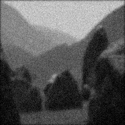
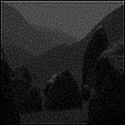
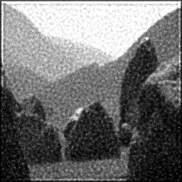
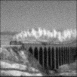
Method: CPU_baseline | Mismatch: nominal (nominal=True, perturbed=False)
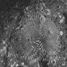
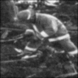
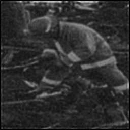
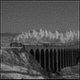
Ground Truth

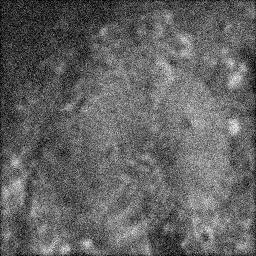
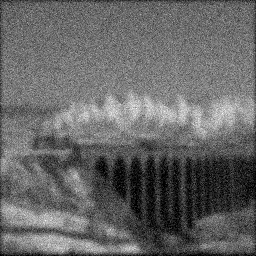
Measurement
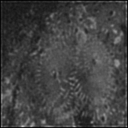
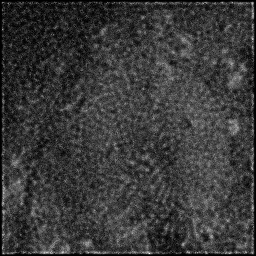
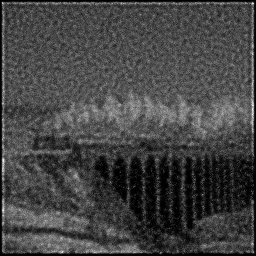
Reconstruction
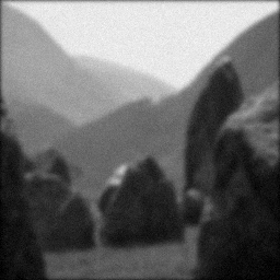
Ground Truth
Measurement
Reconstruction
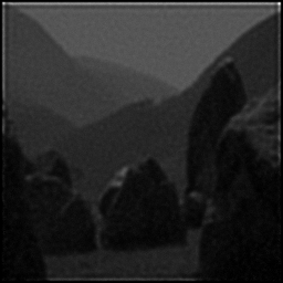
Ground Truth
Measurement (perturbed)

Reconstruction


Mean PSNR Across All Scenes
Per-scene PSNR breakdown (4 scenes)
| Scene | I (PSNR) | I (SSIM) | II (PSNR) | II (SSIM) | III (PSNR) | III (SSIM) |
|---|---|---|---|---|---|---|
| scene_00 | 17.022206064497794 | 0.38380508849556166 | 14.93801985037615 | 0.24399594480247574 | 20.039527108294998 | 0.5012899560940253 |
| scene_01 | 14.231375949985203 | 0.29689664293183293 | 12.92413737908083 | 0.20980780569697918 | 19.225830712320835 | 0.547962131323724 |
| scene_02 | 8.520061941863302 | 0.3871062840596513 | 8.013928482144143 | 0.23077294300010404 | 20.113884181775745 | 0.3416888134023018 |
| scene_03 | 13.297073801541249 | 0.5284335563352818 | 11.66205075678512 | 0.26941399804629346 | 19.61468818224941 | 0.44080752632935544 |
| Mean | 13.267679439471888 | 0.39906039295558193 | 11.884534117096562 | 0.23849767288646312 | 19.748482546160247 | 0.45793710678735156 |
Experimental Setup
Key References
- Minsky, 'Memoir on inventing the confocal microscope', Scanning 10, 128-138 (1988)
- McNally et al., 'Three-dimensional imaging by deconvolution microscopy', Methods 23, 210-217 (1999)
Canonical Datasets
- Cell Tracking Challenge confocal sequences
- BioSR confocal subset
Spec DAG — Forward Model Pipeline
C(PSF_confocal) → D(g, η₃)
Mismatch Parameters
| Symbol | Parameter | Description | Nominal | Perturbed |
|---|---|---|---|---|
| Δph | pinhole | Pinhole diameter error (μm) | 0 | 5.0 |
| Δn | refractive_index | Refractive index mismatch | 1.515 | 1.52 |
| α_b | photobleaching | Photobleaching rate error (%) | 0 | 5.0 |
Credits System
Spec Primitives Reference (11 primitives)
Free-space or medium propagation kernel (Fresnel, Rayleigh-Sommerfeld).
Spatial or spatio-temporal amplitude modulation (coded aperture, SLM pattern).
Geometric projection operator (Radon transform, fan-beam, cone-beam).
Sampling in the Fourier / k-space domain (MRI, ptychography).
Shift-invariant convolution with a point-spread function (PSF).
Summation along a physical dimension (spectral, temporal, angular).
Sensor readout with gain g and noise model η (Gaussian, Poisson, mixed).
Patterned illumination (block, Hadamard, random) applied to the scene.
Spectral dispersion element (prism, grating) with shift α and aperture a.
Sample or gantry rotation (CT, electron tomography).
Spectral filter or monochromator selecting a wavelength band.