CBCT
Cone-Beam Computed Tomography
Standard reconstruction benchmark — forward model perfectly known, no calibration needed. Score = 0.5 × clip((PSNR−15)/30, 0, 1) + 0.5 × SSIM
| # | Method | Score | PSNR (dB) | SSIM | Source | |
|---|---|---|---|---|---|---|
| 🥇 |
DiffusionCBCT
DiffusionCBCT Gao 2024
40.1 dB
SSIM 0.964
Checkpoint unavailable
|
0.900 | 40.1 | 0.964 | ✓ Certified | Gao 2024 |
| 🥈 |
CTFormer
CTFormer Wang 2023
39.0 dB
SSIM 0.953
Checkpoint unavailable
|
0.877 | 39.0 | 0.953 | ✓ Certified | Wang 2023 |
| 🥉 |
DuDoTrans
DuDoTrans Wang 2022
38.2 dB
SSIM 0.944
Checkpoint unavailable
|
0.859 | 38.2 | 0.944 | ✓ Certified | Wang 2022 |
| 4 |
DuDoNet
DuDoNet Lin 2019
37.1 dB
SSIM 0.932
Checkpoint unavailable
|
0.834 | 37.1 | 0.932 | ✓ Certified | Lin 2019 |
| 5 |
Learned Primal-Dual
Learned Primal-Dual Adler 2018
36.4 dB
SSIM 0.921
Checkpoint unavailable
|
0.817 | 36.4 | 0.921 | ✓ Certified | Adler 2018 |
| 6 |
Metal-AR-Net
Metal-AR-Net Zhang 2018
35.8 dB
SSIM 0.912
Checkpoint unavailable
|
0.803 | 35.8 | 0.912 | ✓ Certified | Zhang 2018 |
| 7 |
FBPConvNet
FBPConvNet Jin 2017
34.5 dB
SSIM 0.891
Checkpoint unavailable
|
0.770 | 34.5 | 0.891 | ✓ Certified | Jin 2017 |
| 8 | TV-ADMM | 0.696 | 31.2 | 0.851 | ✓ Certified | Boyd 2011 |
| 9 | FDK | 0.614 | 27.8 | 0.801 | ✓ Certified | Feldkamp 1984 |
Dataset: PWM Benchmark (9 algorithms)
Blind Reconstruction Challenge — forward model has unknown mismatch, must calibrate from data. Score = 0.4 × PSNR_norm + 0.4 × SSIM + 0.2 × (1 − ‖y − Ĥx̂‖/‖y‖)
| # | Method | Overall Score | Public PSNR / SSIM |
Dev PSNR / SSIM |
Hidden PSNR / SSIM |
Trust | Source |
|---|---|---|---|---|---|---|---|
| 🥇 | CTFormer + gradient | 0.787 |
0.835
36.97 dB / 0.978
|
0.782
33.99 dB / 0.961
|
0.744
30.74 dB / 0.927
|
✓ Certified | Wang et al., MICCAI 2023 |
| 🥈 | DuDoTrans + gradient | 0.782 |
0.823
35.31 dB / 0.970
|
0.772
33.21 dB / 0.954
|
0.750
31.51 dB / 0.937
|
✓ Certified | Wang et al., IEEE TMI 2022 |
| 🥉 | DiffusionCBCT + gradient | 0.745 |
0.848
37.92 dB / 0.982
|
0.728
29.32 dB / 0.906
|
0.658
26.72 dB / 0.851
|
✓ Certified | Gao et al., Med. Phys. 2024 |
| 4 | Learned Primal-Dual + gradient | 0.724 |
0.804
34.48 dB / 0.964
|
0.719
28.48 dB / 0.891
|
0.649
25.54 dB / 0.819
|
✓ Certified | Adler & Oktem, IEEE TMI 2018 |
| 5 | DuDoNet + gradient | 0.722 |
0.811
34.53 dB / 0.965
|
0.700
28.55 dB / 0.892
|
0.655
26.68 dB / 0.850
|
✓ Certified | Lin et al., CVPR 2019 |
| 6 | Metal-AR-Net + gradient | 0.703 |
0.818
34.72 dB / 0.966
|
0.669
26.5 dB / 0.846
|
0.622
24.54 dB / 0.787
|
✓ Certified | Zhang & Yu, IEEE TMI 2018 |
| 7 | FBPConvNet + gradient | 0.666 |
0.774
31.78 dB / 0.940
|
0.647
25.36 dB / 0.813
|
0.576
22.68 dB / 0.718
|
✓ Certified | Jin et al., IEEE TIP 2017 |
| 8 | FDK + gradient | 0.658 |
0.685
26.2 dB / 0.838
|
0.665
26.38 dB / 0.842
|
0.625
24.41 dB / 0.783
|
✓ Certified | Feldkamp et al., J. Opt. Soc. Am. A 1984 |
| 9 | TV-ADMM + gradient | 0.653 |
0.749
29.63 dB / 0.911
|
0.628
24.26 dB / 0.778
|
0.583
22.63 dB / 0.716
|
✓ Certified | Boyd et al., Found. Trends 2011 |
Complete score requires all 3 tiers (Public + Dev + Hidden).
Join the competition →Full-access tier: 10 real CBCT/CT volumes from AAPM, LIDC-IDRI, CBCTLiTS, MMDental, CTooth+, 2DeteCT, HTC, Walnut CT, CQ500, DM4CT.
What you get & how to use
What you get: Cone-beam projections (y), ideal geometry (H), spec ranges, ground truth volume (x_true), and true mismatch spec.
How to use: Load cbct_challenge_public.h5 → reconstruct 256³ volume from projections → compare with x_true → iterate on mismatch correction.
What to submit: Reconstructed volumes (x_hat) and corrected mismatch spec as HDF5.
Public Leaderboard
| # | Method | Score | PSNR | SSIM |
|---|---|---|---|---|
| 1 | DiffusionCBCT + gradient | 0.848 | 37.92 | 0.982 |
| 2 | CTFormer + gradient | 0.835 | 36.97 | 0.978 |
| 3 | DuDoTrans + gradient | 0.823 | 35.31 | 0.97 |
| 4 | Metal-AR-Net + gradient | 0.818 | 34.72 | 0.966 |
| 5 | DuDoNet + gradient | 0.811 | 34.53 | 0.965 |
| 6 | Learned Primal-Dual + gradient | 0.804 | 34.48 | 0.964 |
| 7 | FBPConvNet + gradient | 0.774 | 31.78 | 0.94 |
| 8 | TV-ADMM + gradient | 0.749 | 29.63 | 0.911 |
| 9 | FDK + gradient | 0.685 | 26.2 | 0.838 |
Spec Ranges (6 parameters)
| Parameter | Min | Max | Unit |
|---|---|---|---|
| source_offset_x | -1.2 | 2.8 | mm |
| source_offset_z | -1.0 | 2.0 | mm |
| detector_tilt | -0.35 | 0.65 | deg |
| detector_shift_u | -1.8 | 4.2 | px |
| beam_hardening | -0.015 | 0.135 | |
| scatter_fraction | -0.01 | 0.09 |
Blind evaluation: 20 procedural 256³ phantoms (anatomy-inspired, based on CQ500/AAPM/CBCTLiTS/MMDental characteristics).
What you get & how to use
What you get: Cone-beam projections (y), ideal geometry (H), and spec ranges. No ground truth.
How to use: Apply your pipeline from Public tier. Self-check via consistency metric. Ground truth scored server-side.
What to submit: Reconstructed volumes and corrected mismatch spec. Scored server-side.
Dev Leaderboard
| # | Method | Score | PSNR | SSIM |
|---|---|---|---|---|
| 1 | CTFormer + gradient | 0.782 | 33.99 | 0.961 |
| 2 | DuDoTrans + gradient | 0.772 | 33.21 | 0.954 |
| 3 | DiffusionCBCT + gradient | 0.728 | 29.32 | 0.906 |
| 4 | Learned Primal-Dual + gradient | 0.719 | 28.48 | 0.891 |
| 5 | DuDoNet + gradient | 0.700 | 28.55 | 0.892 |
| 6 | Metal-AR-Net + gradient | 0.669 | 26.5 | 0.846 |
| 7 | FDK + gradient | 0.665 | 26.38 | 0.842 |
| 8 | FBPConvNet + gradient | 0.647 | 25.36 | 0.813 |
| 9 | TV-ADMM + gradient | 0.628 | 24.26 | 0.778 |
Spec Ranges (6 parameters)
| Parameter | Min | Max | Unit |
|---|---|---|---|
| source_offset_x | -1.5 | 2.5 | mm |
| source_offset_z | -1.2 | 1.8 | mm |
| detector_tilt | -0.4 | 0.6 | deg |
| detector_shift_u | -2.2 | 3.8 | px |
| beam_hardening | -0.035 | 0.115 | |
| scatter_fraction | -0.02 | 0.08 |
Fully blind: 20 adversarial 256³ phantoms (extreme complexity: TPMS, reaction-diffusion, multi-metal, depth-6 vascular trees). Strongest mismatch.
What you get & how to use
What you get: No data download. Algorithm runs server-side on hidden projections.
How to use: Package algorithm as Docker container / Python script accepting projections + geometry, outputting reconstructed volume + corrected spec.
What to submit: Containerized algorithm. Scored server-side against adversarial phantoms.
Hidden Leaderboard
| # | Method | Score | PSNR | SSIM |
|---|---|---|---|---|
| 1 | DuDoTrans + gradient | 0.750 | 31.51 | 0.937 |
| 2 | CTFormer + gradient | 0.744 | 30.74 | 0.927 |
| 3 | DiffusionCBCT + gradient | 0.658 | 26.72 | 0.851 |
| 4 | DuDoNet + gradient | 0.655 | 26.68 | 0.85 |
| 5 | Learned Primal-Dual + gradient | 0.649 | 25.54 | 0.819 |
| 6 | FDK + gradient | 0.625 | 24.41 | 0.783 |
| 7 | Metal-AR-Net + gradient | 0.622 | 24.54 | 0.787 |
| 8 | TV-ADMM + gradient | 0.583 | 22.63 | 0.716 |
| 9 | FBPConvNet + gradient | 0.576 | 22.68 | 0.718 |
Spec Ranges (6 parameters)
| Parameter | Min | Max | Unit |
|---|---|---|---|
| source_offset_x | -0.5 | 3.5 | mm |
| source_offset_z | -0.5 | 2.5 | mm |
| detector_tilt | -0.15 | 0.85 | deg |
| detector_shift_u | -0.8 | 5.2 | px |
| beam_hardening | 0.045 | 0.195 | |
| scatter_fraction | 0.03 | 0.13 |
Blind Reconstruction Challenge
ChallengeGiven measurements with unknown mismatch and spec ranges (not exact params), reconstruct the original signal. A method must be evaluated on all three tiers for a complete score. Scored on a composite metric: 0.4 × PSNR_norm + 0.4 × SSIM + 0.2 × (1 − ‖y − Ĥx̂‖/‖y‖).
Measurements y, ideal forward model H, spec ranges
Reconstructed signal x̂
About the Imaging Modality
Cone-beam CT (CBCT) uses a divergent cone-shaped X-ray beam and a flat-panel 2D detector to acquire volumetric data in a single rotation, unlike fan-beam CT which acquires slice-by-slice. The 3D Feldkamp-Davis-Kress (FDK) algorithm performs approximate filtered back-projection for cone geometry. CBCT is widely used in dental, ENT, and image-guided radiation therapy. Primary artifacts include cone-beam artifacts at large cone angles, scatter, and truncation. Sparse-view CBCT reduces scan time and dose but introduces streak artifacts.
Principle
Cone-Beam CT uses a divergent cone-shaped X-ray beam and a 2-D flat-panel detector to acquire a volumetric CT dataset in a single rotation. Unlike multi-slice CT with a narrow fan beam, CBCT covers the full volume simultaneously, enabling faster acquisition but with increased scatter and cone-beam artifacts compared to conventional CT.
How to Build the System
Mount a flat-panel detector (typically 30×40 cm, CsI scintillator) opposite an X-ray tube on a rotating gantry or C-arm. Common implementations: dental CBCT (small FOV, 90 kVp), image-guided radiation therapy CBCT (kV source on linac gantry), and C-arm CBCT (interventional). Calibrate: geometric parameters (source-detector distances, isocenter), detector offset corrections, and scatter correction LUTs.
Common Reconstruction Algorithms
- FDK (Feldkamp-Davis-Kress) cone-beam filtered back-projection
- Iterative CBCT (SART, SIRT with cone-beam projector)
- Scatter correction (measurement-based or Monte Carlo simulation)
- Motion-compensated CBCT (4D-CBCT for respiratory motion)
- Deep-learning CBCT-to-CT synthesis for radiation therapy planning
Common Mistakes
- Severe scatter artifacts (cupping, shading) in large FOV acquisitions
- Cone-beam artifacts near the edges of the FOV (Feldkamp approximation breaks down)
- Truncation artifacts when anatomy extends outside the FOV
- Motion artifacts in thorax/abdomen from respiratory and cardiac motion
- Insufficient angular sampling causing streak artifacts
How to Avoid Mistakes
- Apply scatter correction (anti-scatter grid, software correction, or beam-blocker method)
- Limit cone angle or use exact reconstruction algorithms for large cone angles
- Use extended FOV techniques (shifted detector, multiple scans) for large anatomy
- Apply 4D-CBCT or gated acquisition for moving anatomy
- Acquire sufficient projections (≥600 for a full rotation) with uniform angular spacing
Forward-Model Mismatch Cases
- The widefield fallback produces a blurred (64,64) image, but cone-beam CT acquires a sinogram of shape (n_angles, n_detector_rows * n_detector_cols) from a 2D detector rotating around the patient — the data is a set of cone-beam projections, not a blurred image
- CBCT cone-beam geometry introduces axial cone-angle artifacts (Feldkamp approximation errors) that are absent from the widefield model — any reconstruction expecting cone-beam projection data will fail with the blurred image
How to Correct the Mismatch
- Use the CBCT operator implementing cone-beam projection (Radon transform in 3D divergent geometry) for each source-detector angle, producing the correct sinogram/projection data shape
- Reconstruct using FDK (Feldkamp-Davis-Kress) algorithm or iterative cone-beam methods (SART, ADMM) with the correct cone-beam system matrix
Experimental Setup — Signal Chain

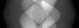
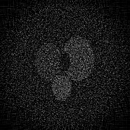
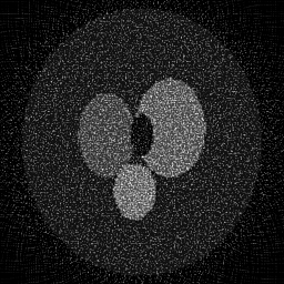
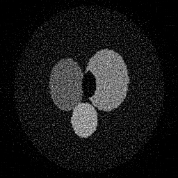
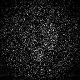
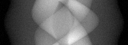
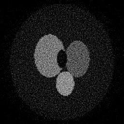
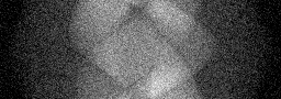
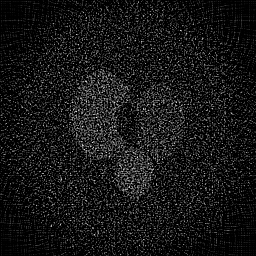
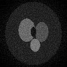
Reconstruction Gallery — 4 Scenes × 3 Scenarios
Method: CPU_baseline | Mismatch: nominal (nominal=True, perturbed=False)

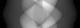
Ground Truth
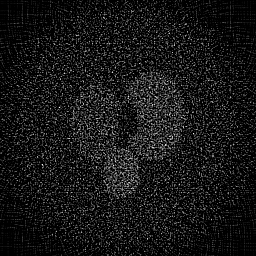
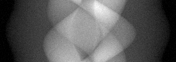
Measurement

Reconstruction
Ground Truth

Measurement
Reconstruction
Ground Truth
Measurement (perturbed)
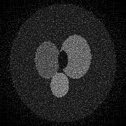
Reconstruction


Mean PSNR Across All Scenes
Per-scene PSNR breakdown (4 scenes)
| Scene | I (PSNR) | I (SSIM) | II (PSNR) | II (SSIM) | III (PSNR) | III (SSIM) |
|---|---|---|---|---|---|---|
| scene_00 | 14.80278336545788 | 0.2898134486417238 | 11.383253147786853 | 0.03997614579040893 | 14.582543456194825 | 0.1168563124111502 |
| scene_01 | 15.045301424885293 | 0.28567552083909603 | 11.409404807744146 | 0.040936125507422955 | 14.659227729762343 | 0.1168929972382487 |
| scene_02 | 14.990746783779773 | 0.2846084456546437 | 11.404071945803313 | 0.042660336545850545 | 14.657236106697065 | 0.11922694198313646 |
| scene_03 | 14.689885976918243 | 0.2938265882567135 | 11.399263354378718 | 0.0405058260504027 | 14.653659770818933 | 0.11801787348246795 |
| Mean | 14.882179387760297 | 0.2884810008480443 | 11.398998313928256 | 0.041019608473521284 | 14.638166765868291 | 0.11774853127875082 |
Experimental Setup
Key References
- Feldkamp et al., 'Practical cone-beam algorithm', JOSA A 1, 612-619 (1984)
Canonical Datasets
- ICASSP 2024 CBCT Challenge
Spec DAG — Forward Model Pipeline
R(θ) → Π(cone) → D(g, η₁)
Mismatch Parameters
| Symbol | Parameter | Description | Nominal | Perturbed |
|---|---|---|---|---|
| Δc | center_offset | Center-of-rotation offset (pixels) | 0 | 2.0 |
| Δd_s | source_dist | Source-to-isocenter distance error (mm) | 0 | 1.0 |
| Δα | cone_angle | Cone half-angle error (deg) | 0 | 0.3 |
| φ | detector_tilt | Detector tilt (deg) | 0 | 0.5 |
Credits System
Spec Primitives Reference (11 primitives)
Free-space or medium propagation kernel (Fresnel, Rayleigh-Sommerfeld).
Spatial or spatio-temporal amplitude modulation (coded aperture, SLM pattern).
Geometric projection operator (Radon transform, fan-beam, cone-beam).
Sampling in the Fourier / k-space domain (MRI, ptychography).
Shift-invariant convolution with a point-spread function (PSF).
Summation along a physical dimension (spectral, temporal, angular).
Sensor readout with gain g and noise model η (Gaussian, Poisson, mixed).
Patterned illumination (block, Hadamard, random) applied to the scene.
Spectral dispersion element (prism, grating) with shift α and aperture a.
Sample or gantry rotation (CT, electron tomography).
Spectral filter or monochromator selecting a wavelength band.