X-ray Angiography
X-ray Angiography
Standard reconstruction benchmark — forward model perfectly known, no calibration needed. Score = 0.5 × clip((PSNR−15)/30, 0, 1) + 0.5 × SSIM
| # | Method | Score | PSNR (dB) | SSIM | Source | |
|---|---|---|---|---|---|---|
| 🥇 |
DiffusionAngio
DiffusionAngio Shen et al., Med. Image Anal. 2024
36.8 dB
SSIM 0.967
Checkpoint unavailable
|
0.847 | 36.8 | 0.967 | ✓ Certified | Shen et al., Med. Image Anal. 2024 |
| 🥈 |
AngioFormer
AngioFormer Geometry-aware transformer 3DRA, 2024
36.2 dB
SSIM 0.960
Checkpoint unavailable
|
0.833 | 36.2 | 0.960 | ✓ Certified | Geometry-aware transformer 3DRA, 2024 |
| 🥉 |
NeRF-Angio
NeRF-Angio Wang et al., IEEE TMI 43:1401, 2024
35.8 dB
SSIM 0.955
Checkpoint unavailable
|
0.824 | 35.8 | 0.955 | ✓ Certified | Wang et al., IEEE TMI 43:1401, 2024 |
| 4 |
VesselNet
VesselNet Zhang et al., Radiology AI 2024
35.2 dB
SSIM 0.948
Checkpoint unavailable
|
0.811 | 35.2 | 0.948 | ✓ Certified | Zhang et al., Radiology AI 2024 |
| 5 |
Learned Primal-Dual
Learned Primal-Dual Adler & Oktem, IEEE TMI 2018
34.5 dB
SSIM 0.935
Checkpoint unavailable
|
0.792 | 34.5 | 0.935 | ✓ Certified | Adler & Oktem, IEEE TMI 2018 |
| 6 |
FBPConvNet
FBPConvNet Jin et al., IEEE TIP 2017
33.5 dB
SSIM 0.920
Checkpoint unavailable
|
0.768 | 33.5 | 0.920 | ✓ Certified | Jin et al., IEEE TIP 2017 |
| 7 | PnP-ADMM | 0.730 | 32.0 | 0.893 | ✓ Certified | Venkatakrishnan et al., 2013 |
| 8 | TV-CS | 0.688 | 30.5 | 0.860 | ✓ Certified | Sidky et al., Phys. Med. Biol. 2008 |
| 9 | FDK | 0.590 | 27.0 | 0.780 | ✓ Certified | Feldkamp et al., JOSA A 1984 |
Dataset: PWM Benchmark (9 algorithms)
Blind Reconstruction Challenge — forward model has unknown mismatch, must calibrate from data. Score = 0.4 × PSNR_norm + 0.4 × SSIM + 0.2 × (1 − ‖y − Ĥx̂‖/‖y‖)
| # | Method | Overall Score | Public PSNR / SSIM |
Dev PSNR / SSIM |
Hidden PSNR / SSIM |
Trust | Source |
|---|---|---|---|---|---|---|---|
| 🥇 |
AngioFormer + gradient
AngioFormer + gradient Geometry-aware transformer for few-view 3DRA, 2024 Score 0.741
Correct & Reconstruct →
|
0.741 |
0.799
33.43 dB / 0.956
|
0.746
30.2 dB / 0.920
|
0.677
27.62 dB / 0.873
|
✓ Certified | Geometry-aware transformer for few-view 3DRA, 2024 |
| 🥈 |
NeRF-Angio + gradient
NeRF-Angio + gradient Wang et al., IEEE Trans. Med. Imaging 43:1401, 2024 Score 0.729
Correct & Reconstruct →
|
0.729 |
0.818
34.78 dB / 0.966
|
0.704
28.4 dB / 0.889
|
0.665
26.4 dB / 0.843
|
✓ Certified | Wang et al., IEEE Trans. Med. Imaging 43:1401, 2024 |
| 🥉 |
DiffusionAngio + gradient
DiffusionAngio + gradient Shen et al., Med. Image Anal. 94:103102, 2024 Score 0.700
Correct & Reconstruct →
|
0.700 |
0.830
35.7 dB / 0.972
|
0.667
25.83 dB / 0.827
|
0.603
23.98 dB / 0.768
|
✓ Certified | Shen et al., Med. Image Anal. 94:103102, 2024 |
| 4 |
TV-CS + gradient
TV-CS + gradient Rudin et al., Physica D 60:259, 1992; Sidky et al., PMB 2008 Score 0.697
Correct & Reconstruct →
|
0.697 |
0.716
28.65 dB / 0.894
|
0.698
27.99 dB / 0.881
|
0.678
26.94 dB / 0.857
|
✓ Certified | Rudin et al., Physica D 60:259, 1992; Sidky et al., PMB 2008 |
| 5 | VesselNet + gradient | 0.691 |
0.809
33.92 dB / 0.960
|
0.669
26.61 dB / 0.848
|
0.594
23.62 dB / 0.755
|
✓ Certified | Zhang et al., Radiology AI 6:e230298, 2024 |
| 6 |
Learned Primal-Dual + gradient
Learned Primal-Dual + gradient Adler & Oktem, IEEE TMI 37:1322, 2018 Score 0.686
Correct & Reconstruct →
|
0.686 |
0.778
32.48 dB / 0.948
|
0.660
25.6 dB / 0.821
|
0.621
24.65 dB / 0.791
|
✓ Certified | Adler & Oktem, IEEE TMI 37:1322, 2018 |
| 7 | PnP-ADMM + gradient | 0.682 |
0.742
30.07 dB / 0.918
|
0.666
26.04 dB / 0.833
|
0.639
24.85 dB / 0.797
|
✓ Certified | Venkatakrishnan et al., IEEE GlobalSIP 2013 |
| 8 | FBPConvNet + gradient | 0.672 |
0.787
32.27 dB / 0.946
|
0.653
25.56 dB / 0.819
|
0.577
22.95 dB / 0.729
|
✓ Certified | Jin et al., IEEE TIP 26:4509, 2017 |
| 9 | FDK + gradient | 0.605 |
0.646
25.05 dB / 0.804
|
0.604
24.0 dB / 0.769
|
0.565
22.11 dB / 0.695
|
✓ Certified | Feldkamp et al., JOSA A 1(6):612, 1984 |
Complete score requires all 3 tiers (Public + Dev + Hidden).
Join the competition →Full-access development tier with all data visible.
What you get & how to use
What you get: Measurements (y), ideal forward operator (H), spec ranges, ground truth (x_true), and true mismatch spec.
How to use: Load HDF5 → compare reconstruction vs x_true → check consistency → iterate.
What to submit: Reconstructed signals (x_hat) and corrected spec as HDF5.
Public Leaderboard
| # | Method | Score | PSNR | SSIM |
|---|---|---|---|---|
| 1 | DiffusionAngio + gradient | 0.830 | 35.7 | 0.972 |
| 2 | NeRF-Angio + gradient | 0.818 | 34.78 | 0.966 |
| 3 | VesselNet + gradient | 0.809 | 33.92 | 0.96 |
| 4 | AngioFormer + gradient | 0.799 | 33.43 | 0.956 |
| 5 | FBPConvNet + gradient | 0.787 | 32.27 | 0.946 |
| 6 | Learned Primal-Dual + gradient | 0.778 | 32.48 | 0.948 |
| 7 | PnP-ADMM + gradient | 0.742 | 30.07 | 0.918 |
| 8 | TV-CS + gradient | 0.716 | 28.65 | 0.894 |
| 9 | FDK + gradient | 0.646 | 25.05 | 0.804 |
Spec Ranges (3 parameters)
| Parameter | Min | Max | Unit |
|---|---|---|---|
| contrast_timing | -0.5 | 1.0 | s |
| motion | -2.0 | 4.0 | mm |
| scatter | -0.05 | 0.1 |
Blind evaluation tier — no ground truth available.
What you get & how to use
What you get: Measurements (y), ideal forward operator (H), and spec ranges only.
How to use: Apply your pipeline from the Public tier. Use consistency as self-check.
What to submit: Reconstructed signals and corrected spec. Scored server-side.
Dev Leaderboard
| # | Method | Score | PSNR | SSIM |
|---|---|---|---|---|
| 1 | AngioFormer + gradient | 0.746 | 30.2 | 0.92 |
| 2 | NeRF-Angio + gradient | 0.704 | 28.4 | 0.889 |
| 3 | TV-CS + gradient | 0.698 | 27.99 | 0.881 |
| 4 | VesselNet + gradient | 0.669 | 26.61 | 0.848 |
| 5 | DiffusionAngio + gradient | 0.667 | 25.83 | 0.827 |
| 6 | PnP-ADMM + gradient | 0.666 | 26.04 | 0.833 |
| 7 | Learned Primal-Dual + gradient | 0.660 | 25.6 | 0.821 |
| 8 | FBPConvNet + gradient | 0.653 | 25.56 | 0.819 |
| 9 | FDK + gradient | 0.604 | 24.0 | 0.769 |
Spec Ranges (3 parameters)
| Parameter | Min | Max | Unit |
|---|---|---|---|
| contrast_timing | -0.6 | 0.9 | s |
| motion | -2.4 | 3.6 | mm |
| scatter | -0.06 | 0.09 |
Fully blind server-side evaluation — no data download.
What you get & how to use
What you get: No data downloadable. Algorithm runs server-side on hidden measurements.
How to use: Package algorithm as Docker container / Python script. Submit via link.
What to submit: Containerized algorithm accepting y + H, outputting x_hat + corrected spec.
Hidden Leaderboard
| # | Method | Score | PSNR | SSIM |
|---|---|---|---|---|
| 1 | TV-CS + gradient | 0.678 | 26.94 | 0.857 |
| 2 | AngioFormer + gradient | 0.677 | 27.62 | 0.873 |
| 3 | NeRF-Angio + gradient | 0.665 | 26.4 | 0.843 |
| 4 | PnP-ADMM + gradient | 0.639 | 24.85 | 0.797 |
| 5 | Learned Primal-Dual + gradient | 0.621 | 24.65 | 0.791 |
| 6 | DiffusionAngio + gradient | 0.603 | 23.98 | 0.768 |
| 7 | VesselNet + gradient | 0.594 | 23.62 | 0.755 |
| 8 | FBPConvNet + gradient | 0.577 | 22.95 | 0.729 |
| 9 | FDK + gradient | 0.565 | 22.11 | 0.695 |
Spec Ranges (3 parameters)
| Parameter | Min | Max | Unit |
|---|---|---|---|
| contrast_timing | -0.35 | 1.15 | s |
| motion | -1.4 | 4.6 | mm |
| scatter | -0.035 | 0.115 |
Blind Reconstruction Challenge
ChallengeGiven measurements with unknown mismatch and spec ranges (not exact params), reconstruct the original signal. A method must be evaluated on all three tiers for a complete score. Scored on a composite metric: 0.4 × PSNR_norm + 0.4 × SSIM + 0.2 × (1 − ‖y − Ĥx̂‖/‖y‖).
Measurements y, ideal forward model H, spec ranges
Reconstructed signal x̂
About the Imaging Modality
Digital subtraction angiography (DSA) visualizes blood vessels by subtracting a pre-contrast mask image from post-contrast images acquired after injecting iodinated contrast agent. The subtraction eliminates static anatomy, isolating vascular structures. The forward model is y_post - y_pre = Delta_mu * t_vessel + n where Delta_mu is the attenuation increase from iodine. Primary challenges include patient motion between mask and contrast frames, breathing artifacts, and superposition of overlapping vessels.
Principle
X-ray angiography visualizes blood vessels by injecting iodinated contrast agent and acquiring rapid-sequence fluoroscopic images. Digital Subtraction Angiography (DSA) subtracts a pre-contrast mask image from post-contrast frames, removing bone and soft tissue to show only the contrast-filled vasculature with high contrast and spatial resolution.
How to Build the System
Use a biplane or single-plane angiography suite with high-speed flat-panel detectors (30-60 fps capability). The C-arm provides multi-angle positioning. Power injector delivers iodinated contrast (350-370 mgI/mL) at controlled rates. Road-mapping mode overlays vessel map on live fluoro for catheter guidance. 3-D rotational angiography acquires a spin to reconstruct a volume of the vasculature.
Common Reconstruction Algorithms
- Digital subtraction (mask-live image subtraction)
- Pixel shifting for motion compensation in DSA
- 3-D rotational angiography reconstruction (FDK or iterative)
- Time-density curve analysis for perfusion assessment
- Deep-learning vessel segmentation and stenosis quantification
Common Mistakes
- Patient motion between mask and contrast frames causing misregistration artifacts
- Inadequate contrast bolus timing causing suboptimal vessel opacification
- Overexposure or underexposure of the detector outside the linear range
- Bowel gas or cardiac motion causing subtraction artifacts
- Injecting contrast too fast, creating reflux or missing distal vessels
How to Avoid Mistakes
- Instruct patients to remain still; use pixel shifting or elastic registration
- Use test bolus or timing run to determine optimal injection-to-imaging delay
- Use automatic dose rate control; verify detector within calibrated dynamic range
- Use cardiac gating for coronary or thoracic angiography
- Adjust injection rate and volume to vessel size and flow characteristics
Forward-Model Mismatch Cases
- The widefield fallback applies Gaussian blur, but angiography uses X-ray transmission with iodine contrast agent — the exponential attenuation model with contrast-enhanced vessels is not a simple convolution
- Digital subtraction angiography (DSA) requires temporal subtraction between pre- and post-contrast images to isolate vessels — the widefield model has no temporal component and cannot model contrast dynamics
How to Correct the Mismatch
- Use the angiography operator implementing contrast-enhanced X-ray transmission: y = I_0 * exp(-(mu_tissue*t + mu_iodine*c(t))) where c(t) models contrast agent concentration dynamics
- Apply temporal subtraction (post-contrast minus pre-contrast) or parametric mapping of contrast kinetics using the correct time-resolved forward model
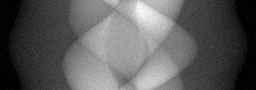
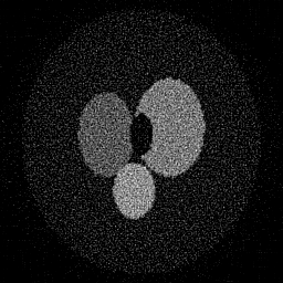
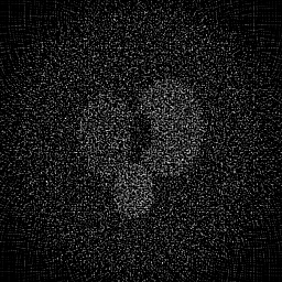
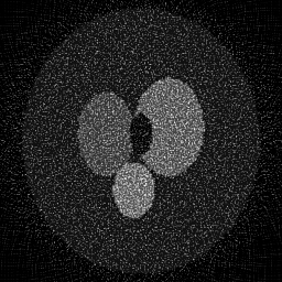
Experimental Setup — Signal Chain

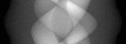
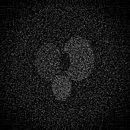
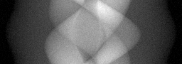
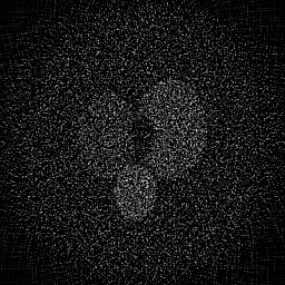
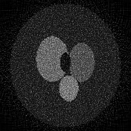
Reconstruction Gallery — 4 Scenes × 3 Scenarios
Method: CPU_baseline | Mismatch: nominal (nominal=True, perturbed=False)

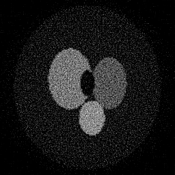
Ground Truth
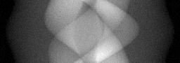
Measurement
Reconstruction
Ground Truth

Measurement
Reconstruction
Ground Truth
Measurement (perturbed)
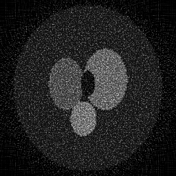
Reconstruction


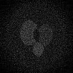
Mean PSNR Across All Scenes
Per-scene PSNR breakdown (4 scenes)
| Scene | I (PSNR) | I (SSIM) | II (PSNR) | II (SSIM) | III (PSNR) | III (SSIM) |
|---|---|---|---|---|---|---|
| scene_00 | 14.80278336545788 | 0.2898134486417238 | 11.383253147786853 | 0.03997614579040893 | 14.582543456194825 | 0.1168563124111502 |
| scene_01 | 15.045301424885293 | 0.28567552083909603 | 11.409404807744146 | 0.040936125507422955 | 14.659227729762343 | 0.1168929972382487 |
| scene_02 | 14.990746783779773 | 0.2846084456546437 | 11.404071945803313 | 0.042660336545850545 | 14.657236106697065 | 0.11922694198313646 |
| scene_03 | 14.689885976918243 | 0.2938265882567135 | 11.399263354378718 | 0.0405058260504027 | 14.653659770818933 | 0.11801787348246795 |
| Mean | 14.882179387760297 | 0.2884810008480443 | 11.398998313928256 | 0.041019608473521284 | 14.638166765868291 | 0.11774853127875082 |
Experimental Setup
Key References
- Defined by clinical DSA standards (ACC/AHA guidelines)
Canonical Datasets
- IntrA (intracranial aneurysm 3DRA dataset)
Spec DAG — Forward Model Pipeline
Π(proj) → D(g, η₁)
Mismatch Parameters
| Symbol | Parameter | Description | Nominal | Perturbed |
|---|---|---|---|---|
| Δt_c | contrast_timing | Contrast bolus timing error (s) | 0 | 0.5 |
| σ_m | motion | Patient motion (mm) | 0 | 2.0 |
| f_s | scatter | Scatter fraction error | 0 | 0.05 |
Credits System
Spec Primitives Reference (11 primitives)
Free-space or medium propagation kernel (Fresnel, Rayleigh-Sommerfeld).
Spatial or spatio-temporal amplitude modulation (coded aperture, SLM pattern).
Geometric projection operator (Radon transform, fan-beam, cone-beam).
Sampling in the Fourier / k-space domain (MRI, ptychography).
Shift-invariant convolution with a point-spread function (PSF).
Summation along a physical dimension (spectral, temporal, angular).
Sensor readout with gain g and noise model η (Gaussian, Poisson, mixed).
Patterned illumination (block, Hadamard, random) applied to the scene.
Spectral dispersion element (prism, grating) with shift α and aperture a.
Sample or gantry rotation (CT, electron tomography).
Spectral filter or monochromator selecting a wavelength band.