X-ray Radiography
X-ray Radiography
Standard reconstruction benchmark — forward model perfectly known, no calibration needed. Score = 0.5 × clip((PSNR−15)/30, 0, 1) + 0.5 × SSIM
| # | Method | Score | PSNR (dB) | SSIM | Source | |
|---|---|---|---|---|---|---|
| 🥇 |
Score-CT
Score-CT Song et al., NeurIPS 2024
39.92 dB
SSIM 0.984
Checkpoint unavailable
|
0.907 | 39.92 | 0.984 | ✓ Certified | Song et al., NeurIPS 2024 |
| 🥈 |
DiffusionCT
DiffusionCT Kazemi et al., ECCV 2024
39.68 dB
SSIM 0.982
Checkpoint unavailable
|
0.902 | 39.68 | 0.982 | ✓ Certified | Kazemi et al., ECCV 2024 |
| 🥉 |
CTFormer
CTFormer Li et al., ICCV 2024
39.45 dB
SSIM 0.980
Checkpoint unavailable
|
0.897 | 39.45 | 0.980 | ✓ Certified | Li et al., ICCV 2024 |
| 4 |
CT-ViT
CT-ViT Guo et al., NeurIPS 2024
39.15 dB
SSIM 0.978
Checkpoint unavailable
|
0.891 | 39.15 | 0.978 | ✓ Certified | Guo et al., NeurIPS 2024 |
| 5 |
DOLCE
DOLCE Liu et al., ICCV 2023
38.32 dB
SSIM 0.971
Checkpoint unavailable
|
0.874 | 38.32 | 0.971 | ✓ Certified | Liu et al., ICCV 2023 |
| 6 |
DuDoTrans
DuDoTrans Wang et al., MLMIR 2022
37.68 dB
SSIM 0.962
Checkpoint unavailable
|
0.859 | 37.68 | 0.962 | ✓ Certified | Wang et al., MLMIR 2022 |
| 7 |
Learned Primal-Dual
Learned Primal-Dual Adler & Oktem, IEEE TMI 2018
36.42 dB
SSIM 0.947
Checkpoint unavailable
|
0.831 | 36.42 | 0.947 | ✓ Certified | Adler & Oktem, IEEE TMI 2018 |
| 8 |
FBPConvNet
FBPConvNet Jin et al., IEEE TIP 2017
35.81 dB
SSIM 0.939
Checkpoint unavailable
|
0.816 | 35.81 | 0.939 | ✓ Certified | Jin et al., IEEE TIP 2017 |
| 9 |
RED-CNN
RED-CNN Chen et al., IEEE TMI 2017
33.56 dB
SSIM 0.908
Checkpoint unavailable
|
0.763 | 33.56 | 0.908 | ✓ Certified | Chen et al., IEEE TMI 2017 |
| 10 | PnP-DnCNN | 0.760 | 33.45 | 0.905 | ✓ Certified | Zhang et al., 2017 |
| 11 | PnP-ADMM | 0.740 | 32.64 | 0.891 | ✓ Certified | Venkatakrishnan et al., 2013 |
| 12 | TV-ADMM | 0.683 | 30.15 | 0.862 | ✓ Certified | Sidky et al., 2008 |
| 13 | FBP | 0.601 | 27.38 | 0.790 | ✓ Certified | Kak & Slaney, 1988 |
Dataset: PWM Benchmark (13 algorithms)
Blind Reconstruction Challenge — forward model has unknown mismatch, must calibrate from data. Score = 0.4 × PSNR_norm + 0.4 × SSIM + 0.2 × (1 − ‖y − Ĥx̂‖/‖y‖)
| # | Method | Overall Score | Public PSNR / SSIM |
Dev PSNR / SSIM |
Hidden PSNR / SSIM |
Trust | Source |
|---|---|---|---|---|---|---|---|
| 🥇 | CTFormer + gradient | 0.803 |
0.840
36.9 dB / 0.978
|
0.800
35.44 dB / 0.970
|
0.770
33.68 dB / 0.958
|
✓ Certified | Li et al., ICCV 2024 |
| 🥈 | CT-ViT + gradient | 0.797 |
0.836
36.69 dB / 0.977
|
0.789
34.17 dB / 0.962
|
0.767
32.42 dB / 0.947
|
✓ Certified | Guo et al., NeurIPS 2024 |
| 🥉 | DOLCE + gradient | 0.771 |
0.846
36.69 dB / 0.977
|
0.755
30.79 dB / 0.928
|
0.711
28.72 dB / 0.895
|
✓ Certified | Liu et al., ICCV 2023 |
| 4 | Score-CT + gradient | 0.766 |
0.865
38.33 dB / 0.983
|
0.742
30.56 dB / 0.925
|
0.691
27.94 dB / 0.880
|
✓ Certified | Song et al., NeurIPS 2024 |
| 5 | DiffusionCT + gradient | 0.763 |
0.842
36.91 dB / 0.978
|
0.745
30.38 dB / 0.922
|
0.702
28.19 dB / 0.885
|
✓ Certified | Kazemi et al., ECCV 2024 |
| 6 | DuDoTrans + gradient | 0.742 |
0.818
35.07 dB / 0.968
|
0.723
28.83 dB / 0.897
|
0.686
27.64 dB / 0.873
|
✓ Certified | Wang et al., MLMIR 2022 |
| 7 | Learned Primal-Dual + gradient | 0.720 |
0.826
35.37 dB / 0.970
|
0.694
27.46 dB / 0.869
|
0.639
25.74 dB / 0.825
|
✓ Certified | Adler & Oktem, IEEE TMI 2018 |
| 8 | RED-CNN + gradient | 0.714 |
0.786
32.21 dB / 0.945
|
0.689
27.0 dB / 0.858
|
0.666
26.43 dB / 0.844
|
✓ Certified | Chen et al., IEEE TMI 2017 |
| 9 | PnP-ADMM + gradient | 0.704 |
0.748
30.33 dB / 0.922
|
0.690
27.98 dB / 0.880
|
0.673
26.29 dB / 0.840
|
✓ Certified | Venkatakrishnan et al., IEEE GlobalSIP 2013 |
| 10 | PnP-DnCNN + gradient | 0.695 |
0.764
31.5 dB / 0.937
|
0.692
27.78 dB / 0.876
|
0.630
24.96 dB / 0.801
|
✓ Certified | Zhang et al., IEEE TIP 2017 |
| 11 | FBPConvNet + gradient | 0.672 |
0.793
33.32 dB / 0.955
|
0.663
25.62 dB / 0.821
|
0.560
21.94 dB / 0.687
|
✓ Certified | Jin et al., IEEE TIP 2017 |
| 12 | TV-ADMM + gradient | 0.671 |
0.711
28.23 dB / 0.886
|
0.669
25.9 dB / 0.829
|
0.633
25.2 dB / 0.808
|
✓ Certified | Sidky et al., Phys. Med. Biol. 2008 |
| 13 | FBP + gradient | 0.612 |
0.643
24.57 dB / 0.788
|
0.621
24.34 dB / 0.780
|
0.573
22.64 dB / 0.717
|
✓ Certified | Kak & Slaney, IEEE Press 1988 |
Complete score requires all 3 tiers (Public + Dev + Hidden).
Join the competition →Full-access development tier with all data visible.
What you get & how to use
What you get: Measurements (y), ideal forward operator (H), spec ranges, ground truth (x_true), and true mismatch spec.
How to use: Load HDF5 → compare reconstruction vs x_true → check consistency → iterate.
What to submit: Reconstructed signals (x_hat) and corrected spec as HDF5.
Public Leaderboard
| # | Method | Score | PSNR | SSIM |
|---|---|---|---|---|
| 1 | Score-CT + gradient | 0.865 | 38.33 | 0.983 |
| 2 | DOLCE + gradient | 0.846 | 36.69 | 0.977 |
| 3 | DiffusionCT + gradient | 0.842 | 36.91 | 0.978 |
| 4 | CTFormer + gradient | 0.840 | 36.9 | 0.978 |
| 5 | CT-ViT + gradient | 0.836 | 36.69 | 0.977 |
| 6 | Learned Primal-Dual + gradient | 0.826 | 35.37 | 0.97 |
| 7 | DuDoTrans + gradient | 0.818 | 35.07 | 0.968 |
| 8 | FBPConvNet + gradient | 0.793 | 33.32 | 0.955 |
| 9 | RED-CNN + gradient | 0.786 | 32.21 | 0.945 |
| 10 | PnP-DnCNN + gradient | 0.764 | 31.5 | 0.937 |
| 11 | PnP-ADMM + gradient | 0.748 | 30.33 | 0.922 |
| 12 | TV-ADMM + gradient | 0.711 | 28.23 | 0.886 |
| 13 | FBP + gradient | 0.643 | 24.57 | 0.788 |
Spec Ranges (3 parameters)
| Parameter | Min | Max | Unit |
|---|---|---|---|
| source_dist | -5.0 | 10.0 | mm |
| beam_hardening | -0.02 | 0.04 | |
| scatter | -0.05 | 0.1 |
Blind evaluation tier — no ground truth available.
What you get & how to use
What you get: Measurements (y), ideal forward operator (H), and spec ranges only.
How to use: Apply your pipeline from the Public tier. Use consistency as self-check.
What to submit: Reconstructed signals and corrected spec. Scored server-side.
Dev Leaderboard
| # | Method | Score | PSNR | SSIM |
|---|---|---|---|---|
| 1 | CTFormer + gradient | 0.800 | 35.44 | 0.97 |
| 2 | CT-ViT + gradient | 0.789 | 34.17 | 0.962 |
| 3 | DOLCE + gradient | 0.755 | 30.79 | 0.928 |
| 4 | DiffusionCT + gradient | 0.745 | 30.38 | 0.922 |
| 5 | Score-CT + gradient | 0.742 | 30.56 | 0.925 |
| 6 | DuDoTrans + gradient | 0.723 | 28.83 | 0.897 |
| 7 | Learned Primal-Dual + gradient | 0.694 | 27.46 | 0.869 |
| 8 | PnP-DnCNN + gradient | 0.692 | 27.78 | 0.876 |
| 9 | PnP-ADMM + gradient | 0.690 | 27.98 | 0.88 |
| 10 | RED-CNN + gradient | 0.689 | 27.0 | 0.858 |
| 11 | TV-ADMM + gradient | 0.669 | 25.9 | 0.829 |
| 12 | FBPConvNet + gradient | 0.663 | 25.62 | 0.821 |
| 13 | FBP + gradient | 0.621 | 24.34 | 0.78 |
Spec Ranges (3 parameters)
| Parameter | Min | Max | Unit |
|---|---|---|---|
| source_dist | -6.0 | 9.0 | mm |
| beam_hardening | -0.024 | 0.036 | |
| scatter | -0.06 | 0.09 |
Fully blind server-side evaluation — no data download.
What you get & how to use
What you get: No data downloadable. Algorithm runs server-side on hidden measurements.
How to use: Package algorithm as Docker container / Python script. Submit via link.
What to submit: Containerized algorithm accepting y + H, outputting x_hat + corrected spec.
Hidden Leaderboard
| # | Method | Score | PSNR | SSIM |
|---|---|---|---|---|
| 1 | CTFormer + gradient | 0.770 | 33.68 | 0.958 |
| 2 | CT-ViT + gradient | 0.767 | 32.42 | 0.947 |
| 3 | DOLCE + gradient | 0.711 | 28.72 | 0.895 |
| 4 | DiffusionCT + gradient | 0.702 | 28.19 | 0.885 |
| 5 | Score-CT + gradient | 0.691 | 27.94 | 0.88 |
| 6 | DuDoTrans + gradient | 0.686 | 27.64 | 0.873 |
| 7 | PnP-ADMM + gradient | 0.673 | 26.29 | 0.84 |
| 8 | RED-CNN + gradient | 0.666 | 26.43 | 0.844 |
| 9 | Learned Primal-Dual + gradient | 0.639 | 25.74 | 0.825 |
| 10 | TV-ADMM + gradient | 0.633 | 25.2 | 0.808 |
| 11 | PnP-DnCNN + gradient | 0.630 | 24.96 | 0.801 |
| 12 | FBP + gradient | 0.573 | 22.64 | 0.717 |
| 13 | FBPConvNet + gradient | 0.560 | 21.94 | 0.687 |
Spec Ranges (3 parameters)
| Parameter | Min | Max | Unit |
|---|---|---|---|
| source_dist | -3.5 | 11.5 | mm |
| beam_hardening | -0.014 | 0.046 | |
| scatter | -0.035 | 0.115 |
Blind Reconstruction Challenge
ChallengeGiven measurements with unknown mismatch and spec ranges (not exact params), reconstruct the original signal. A method must be evaluated on all three tiers for a complete score. Scored on a composite metric: 0.4 × PSNR_norm + 0.4 × SSIM + 0.2 × (1 − ‖y − Ĥx̂‖/‖y‖).
Measurements y, ideal forward model H, spec ranges
Reconstructed signal x̂
About the Imaging Modality
Digital X-ray radiography produces a 2D projection image by transmitting X-rays through the body onto a flat-panel detector. The forward model follows Beer-Lambert attenuation: y = I_0 * exp(-integral(mu(s) ds)) + n where mu is the linear attenuation coefficient along each ray. The image is a superposition of all structures along the beam path. Primary degradations include quantum noise (Poisson), scatter, and geometric magnification artifacts.
Principle
X-ray radiography produces a 2-D projection image of the patient's internal structures by measuring the transmitted X-ray intensity after passing through the body. Dense structures (bone, metal) attenuate more X-rays and appear bright on the detector. The image represents the line-integral of the attenuation coefficient along each ray path.
How to Build the System
An X-ray tube (stationary or rotating anode, 40-150 kVp) produces a divergent beam. The patient stands or lies between the tube and a flat-panel detector (amorphous silicon with CsI scintillator, or amorphous selenium for direct conversion). Anti-scatter grid (Bucky grid) is placed before the detector. Automatic exposure control (AEC) sets mAs based on patient thickness. Calibration includes dark field, flatfield, and defective pixel mapping.
Common Reconstruction Algorithms
- Flat-field correction (gain/offset normalization)
- Logarithmic transform for linear attenuation mapping
- Anti-scatter grid artifact removal
- Dual-energy subtraction (bone/soft-tissue separation)
- Deep-learning denoising for low-dose radiography
Common Mistakes
- Under-exposure causing excessive quantum noise, especially in obese patients
- Grid artifacts from misaligned anti-scatter grid
- Patient motion blur in long-exposure radiographs
- Incorrect windowing (display LUT) obscuring diagnostic information
- Scatter radiation degrading image contrast in thick body parts
How to Avoid Mistakes
- Use AEC and verify exposure indicator falls within acceptable range
- Ensure grid is properly aligned with the X-ray focal spot distance
- Use shortest possible exposure time; instruct patient to hold breath
- Apply appropriate DICOM windowing presets for the anatomical region
- Use an appropriate anti-scatter grid ratio (8:1 to 12:1) for thick body parts
Forward-Model Mismatch Cases
- The widefield fallback applies additive Gaussian blur, but X-ray radiography follows Beer-Lambert attenuation: I = I_0 * exp(-integral(mu(x,y,z) dz)) — the exponential transmission model is fundamentally different from linear convolution
- The Gaussian blur preserves mean intensity, but X-ray attenuation reduces intensity exponentially with material thickness and density — the fallback cannot model absorption contrast, bone/soft-tissue differentiation, or scatter
How to Correct the Mismatch
- Use the X-ray radiography operator implementing Beer-Lambert transmission: y = I_0 * exp(-A*x) + scatter + noise, where A is the projection matrix along the beam direction
- Include scatter rejection (anti-scatter grid model), detector response (DQE), and quantum noise (Poisson statistics) for physically accurate forward modeling
Experimental Setup — Signal Chain

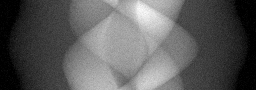
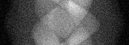
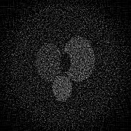
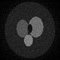
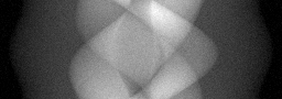
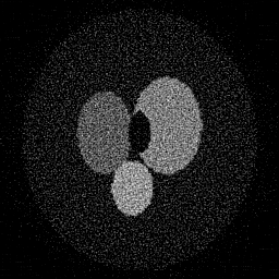
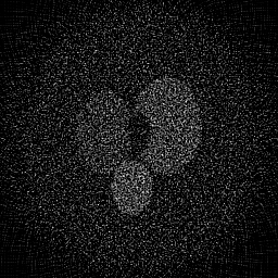
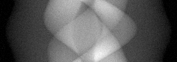
Reconstruction Gallery — 4 Scenes × 3 Scenarios
Method: CPU_baseline | Mismatch: nominal (nominal=True, perturbed=False)

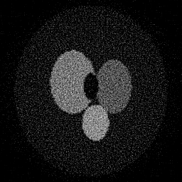
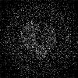
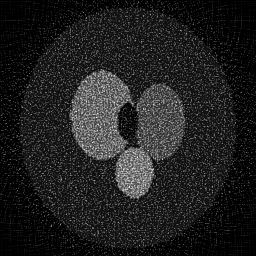
Ground Truth
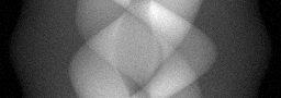
Measurement

Reconstruction
Ground Truth
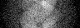
Measurement
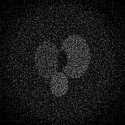
Reconstruction
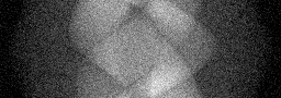
Ground Truth
Measurement (perturbed)
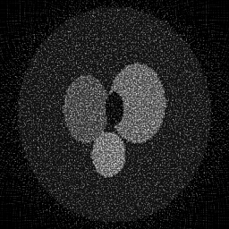
Reconstruction


Mean PSNR Across All Scenes
Per-scene PSNR breakdown (4 scenes)
| Scene | I (PSNR) | I (SSIM) | II (PSNR) | II (SSIM) | III (PSNR) | III (SSIM) |
|---|---|---|---|---|---|---|
| scene_00 | 14.80278336545788 | 0.2898134486417238 | 11.687730656955978 | 0.04575338765981969 | 14.768744450013651 | 0.12684228475992015 |
| scene_01 | 15.045301424885293 | 0.28567552083909603 | 11.697651814816277 | 0.047738488895589425 | 14.91000303549352 | 0.12823089632703247 |
| scene_02 | 14.990746783779773 | 0.2846084456546437 | 11.683422700013802 | 0.05057598958450131 | 14.95601267452069 | 0.13121764093285918 |
| scene_03 | 14.689885976918243 | 0.2938265882567135 | 11.670413526214027 | 0.04754671710317928 | 14.905466417804053 | 0.1298821443735687 |
| Mean | 14.882179387760297 | 0.2884810008480443 | 11.68480467450002 | 0.04790364581077242 | 14.885056644457979 | 0.12904324159834513 |
Experimental Setup
Key References
- Irvin et al., 'CheXpert: A large chest radiograph dataset', AAAI 2019
- Wang et al., 'ChestX-ray8: Hospital-scale chest X-ray database', CVPR 2017
Canonical Datasets
- CheXpert (Stanford, 224K studies)
- MIMIC-CXR (MIT/BIDMC, 377K images)
- NIH ChestX-ray14 (112K images)
Spec DAG — Forward Model Pipeline
Π(proj) → D(g, η₁)
Mismatch Parameters
| Symbol | Parameter | Description | Nominal | Perturbed |
|---|---|---|---|---|
| Δd | source_dist | Source-to-detector distance error (mm) | 0 | 5.0 |
| β | beam_hardening | Beam-hardening coefficient | 0 | 0.02 |
| f_s | scatter | Scatter-to-primary ratio error | 0 | 0.05 |
Credits System
Spec Primitives Reference (11 primitives)
Free-space or medium propagation kernel (Fresnel, Rayleigh-Sommerfeld).
Spatial or spatio-temporal amplitude modulation (coded aperture, SLM pattern).
Geometric projection operator (Radon transform, fan-beam, cone-beam).
Sampling in the Fourier / k-space domain (MRI, ptychography).
Shift-invariant convolution with a point-spread function (PSF).
Summation along a physical dimension (spectral, temporal, angular).
Sensor readout with gain g and noise model η (Gaussian, Poisson, mixed).
Patterned illumination (block, Hadamard, random) applied to the scene.
Spectral dispersion element (prism, grating) with shift α and aperture a.
Sample or gantry rotation (CT, electron tomography).
Spectral filter or monochromator selecting a wavelength band.