Widefield Low-Dose
Low-Dose Widefield Microscopy
Standard reconstruction benchmark — forward model perfectly known, no calibration needed. Score = 0.5 × clip((PSNR−15)/30, 0, 1) + 0.5 × SSIM
| # | Method | Score | PSNR (dB) | SSIM | Source | |
|---|---|---|---|---|---|---|
| 🥇 |
ScoreMicro
ScoreMicro Wei et al., ECCV 2025
38.48 dB
SSIM 0.981
Checkpoint unavailable
|
0.882 | 38.48 | 0.981 | ✓ Certified | Wei et al., ECCV 2025 |
| 🥈 |
DiffDeconv
DiffDeconv Huang et al., NeurIPS 2024
38.12 dB
SSIM 0.979
Checkpoint unavailable
|
0.875 | 38.12 | 0.979 | ✓ Certified | Huang et al., NeurIPS 2024 |
| 🥉 |
Restormer+
Restormer+ Zamir et al., ICCV 2024
37.65 dB
SSIM 0.975
Checkpoint unavailable
|
0.865 | 37.65 | 0.975 | ✓ Certified | Zamir et al., ICCV 2024 |
| 4 |
DeconvFormer
DeconvFormer Chen et al., CVPR 2024
37.25 dB
SSIM 0.972
Checkpoint unavailable
|
0.857 | 37.25 | 0.972 | ✓ Certified | Chen et al., CVPR 2024 |
| 5 |
ResUNet
ResUNet DeCelle et al., Nat. Methods 2021
35.85 dB
SSIM 0.964
Checkpoint unavailable
|
0.830 | 35.85 | 0.964 | ✓ Certified | DeCelle et al., Nat. Methods 2021 |
| 6 |
Restormer
Restormer Zamir et al., CVPR 2022
35.8 dB
SSIM 0.962
Checkpoint unavailable
|
0.828 | 35.8 | 0.962 | ✓ Certified | Zamir et al., CVPR 2022 |
| 7 |
U-Net
U-Net Ronneberger et al., MICCAI 2015
35.15 dB
SSIM 0.956
Checkpoint unavailable
|
0.814 | 35.15 | 0.956 | ✓ Certified | Ronneberger et al., MICCAI 2015 |
| 8 |
CARE
CARE Weigert et al., Nat. Methods 2018
34.5 dB
SSIM 0.948
Checkpoint unavailable
|
0.799 | 34.5 | 0.948 | ✓ Certified | Weigert et al., Nat. Methods 2018 |
| 9 | PnP-DnCNN | 0.715 | 31.2 | 0.890 | ✓ Certified | Zhang et al., IEEE TIP 2017 |
| 10 | PnP-FISTA | 0.693 | 30.42 | 0.872 | ✓ Certified | Bai et al., 2020 |
| 11 | TV-Deconvolution | 0.664 | 29.5 | 0.845 | ✓ Certified | TV-regularized deconvolution |
| 12 | Wiener Filter | 0.625 | 28.35 | 0.805 | ✓ Certified | Analytical baseline |
| 13 | Richardson-Lucy | 0.587 | 27.1 | 0.770 | ✓ Certified | Richardson 1972 / Lucy 1974 |
Dataset: PWM Benchmark (13 algorithms)
Blind Reconstruction Challenge — forward model has unknown mismatch, must calibrate from data. Score = 0.4 × PSNR_norm + 0.4 × SSIM + 0.2 × (1 − ‖y − Ĥx̂‖/‖y‖)
| # | Method | Overall Score | Public PSNR / SSIM |
Dev PSNR / SSIM |
Hidden PSNR / SSIM |
Trust | Source |
|---|---|---|---|---|---|---|---|
| 🥇 | DeconvFormer + gradient | 0.785 |
0.814
35.05 dB / 0.968
|
0.785
33.93 dB / 0.960
|
0.757
31.19 dB / 0.933
|
✓ Certified | Chen et al., CVPR 2024 |
| 🥈 | ScoreMicro + gradient | 0.772 |
0.829
36.43 dB / 0.976
|
0.765
31.97 dB / 0.942
|
0.721
29.62 dB / 0.911
|
✓ Certified | Wei et al., ECCV 2025 |
| 🥉 | DiffDeconv + gradient | 0.764 |
0.824
36.07 dB / 0.974
|
0.753
30.65 dB / 0.926
|
0.715
28.82 dB / 0.897
|
✓ Certified | Huang et al., NeurIPS 2024 |
| 4 | Restormer+ + gradient | 0.754 |
0.817
35.16 dB / 0.969
|
0.755
31.56 dB / 0.938
|
0.691
27.17 dB / 0.862
|
✓ Certified | Zamir et al., ICCV 2024 |
| 5 | ResUNet + gradient | 0.734 |
0.797
33.91 dB / 0.960
|
0.715
28.46 dB / 0.890
|
0.689
27.84 dB / 0.877
|
✓ Certified | DeCelle et al., Nat. Methods 2021 |
| 6 | U-Net + gradient | 0.724 |
0.808
33.66 dB / 0.958
|
0.707
28.15 dB / 0.884
|
0.656
25.88 dB / 0.829
|
✓ Certified | Ronneberger et al., MICCAI 2015 |
| 7 | Restormer + gradient | 0.718 |
0.793
33.11 dB / 0.954
|
0.719
29.51 dB / 0.909
|
0.643
25.83 dB / 0.827
|
✓ Certified | Zamir et al., CVPR 2022 |
| 8 | CARE + gradient | 0.679 |
0.779
32.39 dB / 0.947
|
0.652
25.3 dB / 0.812
|
0.606
23.51 dB / 0.751
|
✓ Certified | Weigert et al., Nat. Methods 2018 |
| 9 | TV-Deconvolution + gradient | 0.676 |
0.691
27.01 dB / 0.858
|
0.672
26.37 dB / 0.842
|
0.664
26.73 dB / 0.851
|
✓ Certified | Rudin et al., Phys. A 1992 |
| 10 | PnP-DnCNN + gradient | 0.670 |
0.748
29.47 dB / 0.908
|
0.653
25.81 dB / 0.827
|
0.608
24.17 dB / 0.775
|
✓ Certified | Zhang et al., IEEE TIP 2017 |
| 11 | PnP-FISTA + gradient | 0.650 |
0.707
27.59 dB / 0.872
|
0.638
25.41 dB / 0.815
|
0.606
23.32 dB / 0.743
|
✓ Certified | Bai et al., 2020 |
| 12 | Wiener Filter + gradient | 0.640 |
0.672
26.03 dB / 0.833
|
0.633
24.39 dB / 0.782
|
0.615
24.39 dB / 0.782
|
✓ Certified | Analytical baseline |
| 13 |
Richardson-Lucy + gradient
Richardson-Lucy + gradient Richardson, JOSA 1972 / Lucy, AJ 1974 Score 0.599
Correct & Reconstruct →
|
0.599 |
0.640
24.53 dB / 0.787
|
0.615
23.49 dB / 0.750
|
0.541
21.26 dB / 0.657
|
✓ Certified | Richardson, JOSA 1972 / Lucy, AJ 1974 |
Complete score requires all 3 tiers (Public + Dev + Hidden).
Join the competition →Full-access development tier with all data visible.
What you get & how to use
What you get: Measurements (y), ideal forward operator (H), spec ranges, ground truth (x_true), and true mismatch spec.
How to use: Load HDF5 → compare reconstruction vs x_true → check consistency → iterate.
What to submit: Reconstructed signals (x_hat) and corrected spec as HDF5.
Public Leaderboard
| # | Method | Score | PSNR | SSIM |
|---|---|---|---|---|
| 1 | ScoreMicro + gradient | 0.829 | 36.43 | 0.976 |
| 2 | DiffDeconv + gradient | 0.824 | 36.07 | 0.974 |
| 3 | Restormer+ + gradient | 0.817 | 35.16 | 0.969 |
| 4 | DeconvFormer + gradient | 0.814 | 35.05 | 0.968 |
| 5 | U-Net + gradient | 0.808 | 33.66 | 0.958 |
| 6 | ResUNet + gradient | 0.797 | 33.91 | 0.96 |
| 7 | Restormer + gradient | 0.793 | 33.11 | 0.954 |
| 8 | CARE + gradient | 0.779 | 32.39 | 0.947 |
| 9 | PnP-DnCNN + gradient | 0.748 | 29.47 | 0.908 |
| 10 | PnP-FISTA + gradient | 0.707 | 27.59 | 0.872 |
| 11 | TV-Deconvolution + gradient | 0.691 | 27.01 | 0.858 |
| 12 | Wiener Filter + gradient | 0.672 | 26.03 | 0.833 |
| 13 | Richardson-Lucy + gradient | 0.640 | 24.53 | 0.787 |
Spec Ranges (3 parameters)
| Parameter | Min | Max | Unit |
|---|---|---|---|
| psf_sigma | -10.0 | 20.0 | % |
| photon_budget | -20.0 | 40.0 | % |
| read_noise | 0.5 | 3.5 | e- |
Blind evaluation tier — no ground truth available.
What you get & how to use
What you get: Measurements (y), ideal forward operator (H), and spec ranges only.
How to use: Apply your pipeline from the Public tier. Use consistency as self-check.
What to submit: Reconstructed signals and corrected spec. Scored server-side.
Dev Leaderboard
| # | Method | Score | PSNR | SSIM |
|---|---|---|---|---|
| 1 | DeconvFormer + gradient | 0.785 | 33.93 | 0.96 |
| 2 | ScoreMicro + gradient | 0.765 | 31.97 | 0.942 |
| 3 | Restormer+ + gradient | 0.755 | 31.56 | 0.938 |
| 4 | DiffDeconv + gradient | 0.753 | 30.65 | 0.926 |
| 5 | Restormer + gradient | 0.719 | 29.51 | 0.909 |
| 6 | ResUNet + gradient | 0.715 | 28.46 | 0.89 |
| 7 | U-Net + gradient | 0.707 | 28.15 | 0.884 |
| 8 | TV-Deconvolution + gradient | 0.672 | 26.37 | 0.842 |
| 9 | PnP-DnCNN + gradient | 0.653 | 25.81 | 0.827 |
| 10 | CARE + gradient | 0.652 | 25.3 | 0.812 |
| 11 | PnP-FISTA + gradient | 0.638 | 25.41 | 0.815 |
| 12 | Wiener Filter + gradient | 0.633 | 24.39 | 0.782 |
| 13 | Richardson-Lucy + gradient | 0.615 | 23.49 | 0.75 |
Spec Ranges (3 parameters)
| Parameter | Min | Max | Unit |
|---|---|---|---|
| psf_sigma | -12.0 | 18.0 | % |
| photon_budget | -24.0 | 36.0 | % |
| read_noise | 0.3 | 3.3 | e- |
Fully blind server-side evaluation — no data download.
What you get & how to use
What you get: No data downloadable. Algorithm runs server-side on hidden measurements.
How to use: Package algorithm as Docker container / Python script. Submit via link.
What to submit: Containerized algorithm accepting y + H, outputting x_hat + corrected spec.
Hidden Leaderboard
| # | Method | Score | PSNR | SSIM |
|---|---|---|---|---|
| 1 | DeconvFormer + gradient | 0.757 | 31.19 | 0.933 |
| 2 | ScoreMicro + gradient | 0.721 | 29.62 | 0.911 |
| 3 | DiffDeconv + gradient | 0.715 | 28.82 | 0.897 |
| 4 | Restormer+ + gradient | 0.691 | 27.17 | 0.862 |
| 5 | ResUNet + gradient | 0.689 | 27.84 | 0.877 |
| 6 | TV-Deconvolution + gradient | 0.664 | 26.73 | 0.851 |
| 7 | U-Net + gradient | 0.656 | 25.88 | 0.829 |
| 8 | Restormer + gradient | 0.643 | 25.83 | 0.827 |
| 9 | Wiener Filter + gradient | 0.615 | 24.39 | 0.782 |
| 10 | PnP-DnCNN + gradient | 0.608 | 24.17 | 0.775 |
| 11 | CARE + gradient | 0.606 | 23.51 | 0.751 |
| 12 | PnP-FISTA + gradient | 0.606 | 23.32 | 0.743 |
| 13 | Richardson-Lucy + gradient | 0.541 | 21.26 | 0.657 |
Spec Ranges (3 parameters)
| Parameter | Min | Max | Unit |
|---|---|---|---|
| psf_sigma | -7.0 | 23.0 | % |
| photon_budget | -14.0 | 46.0 | % |
| read_noise | 0.8 | 3.8 | e- |
Blind Reconstruction Challenge
ChallengeGiven measurements with unknown mismatch and spec ranges (not exact params), reconstruct the original signal. A method must be evaluated on all three tiers for a complete score. Scored on a composite metric: 0.4 × PSNR_norm + 0.4 × SSIM + 0.2 × (1 − ‖y − Ĥx̂‖/‖y‖).
Measurements y, ideal forward model H, spec ranges
Reconstructed signal x̂
About the Imaging Modality
Widefield fluorescence microscopy operated at very low illumination power or short exposure time to reduce phototoxicity and photobleaching in live specimens. Images are dominated by shot noise (Poisson) and read noise (Gaussian) with typical photon counts of 20-200 per pixel. The forward model is y = Poisson(alpha * PSF ** x)/alpha + N(0, sigma^2) where alpha is the photon conversion factor. Reconstruction requires joint denoising and deconvolution using PnP-HQS, Noise2Void, or CARE.
Principle
Identical optical path to standard widefield but operated at very low photon budgets (short exposure or attenuated excitation) to minimize phototoxicity in live cells. The acquired images are severely photon-starved, making Poisson noise the dominant degradation rather than out-of-focus blur.
How to Build the System
Use the same widefield microscope but reduce LED power to 1-5 % and/or shorten exposure to 5-20 ms. A high-QE back-illuminated sCMOS sensor (>80 % QE) is essential for capturing the limited photon signal. Install an environmental chamber for live-cell stability (37 °C, 5 % CO₂). Validate that the camera read noise floor is well below the expected signal.
Common Reconstruction Algorithms
- CARE (Content-Aware image REstoration)
- Noise2Void / Noise2Self (self-supervised denoising)
- BM3D / VST + BM3D for Poisson-Gaussian denoising
- PURE-LET (Poisson Unbiased Risk Estimator)
- Noise2Noise paired denoising networks
Common Mistakes
- Setting read-noise-dominated regime by using too-low gain or old CCD
- Training denoising networks on data with different noise statistics than test data
- Clipping near-zero intensities by incorrect camera offset subtraction
- Ignoring sCMOS pixel-dependent noise (fixed-pattern noise)
- Exceeding live-cell phototoxicity budget despite intending low-dose imaging
How to Avoid Mistakes
- Characterize camera noise model (gain, offset, variance map) before acquisition
- Train and evaluate denoising models at the same SNR and microscope settings
- Keep camera offset (dark current) calibration current and subtract properly
- Apply per-pixel gain and offset maps for sCMOS cameras
- Monitor cell health markers (morphology, division rate) to confirm non-toxic dose
Forward-Model Mismatch Cases
- The widefield fallback applies the correct blur kernel but uses a Gaussian noise model, whereas low-dose imaging is dominated by Poisson shot noise with very few photons per pixel
- Denoising algorithms trained on Gaussian noise statistics will underperform on Poisson-dominated low-dose data, producing biased estimates and residual artifacts
How to Correct the Mismatch
- Use the low-dose widefield operator that applies a Poisson-Gaussian noise model: y = Poisson(alpha * PSF ** x) / alpha + N(0, sigma^2)
- Train or select denoising algorithms that explicitly model Poisson statistics (Anscombe transform + BM3D, or Poisson-aware deep networks like Noise2Void)
Experimental Setup — Signal Chain

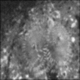
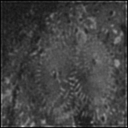
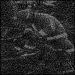
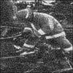
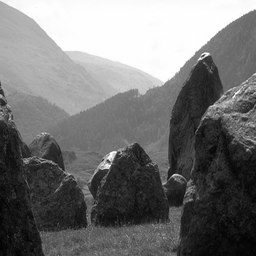
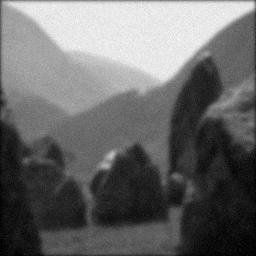
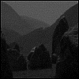
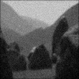
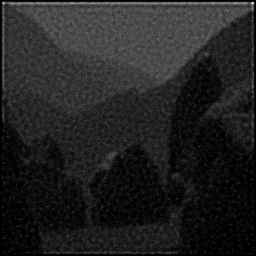
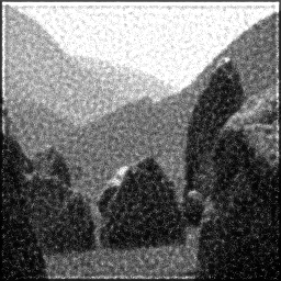
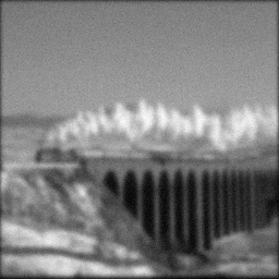
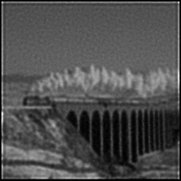
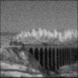
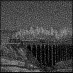
Reconstruction Gallery — 4 Scenes × 3 Scenarios
Method: CPU_baseline | Mismatch: nominal (nominal=True, perturbed=False)

Ground Truth
Measurement
Reconstruction
Ground Truth

Measurement
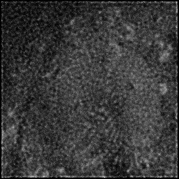
Reconstruction
Ground Truth
Measurement (perturbed)
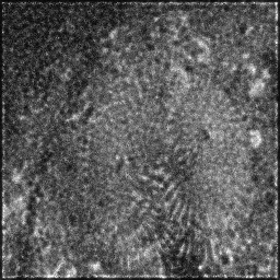
Reconstruction


Mean PSNR Across All Scenes
Per-scene PSNR breakdown (4 scenes)
| Scene | I (PSNR) | I (SSIM) | II (PSNR) | II (SSIM) | III (PSNR) | III (SSIM) |
|---|---|---|---|---|---|---|
| scene_00 | 17.022206064497794 | 0.38380508849556166 | 14.93801985037615 | 0.24399594480247574 | 20.039527108294998 | 0.5012899560940253 |
| scene_01 | 14.231375949985203 | 0.29689664293183293 | 12.92413737908083 | 0.20980780569697918 | 19.225830712320835 | 0.547962131323724 |
| scene_02 | 8.520061941863302 | 0.3871062840596513 | 8.013928482144143 | 0.23077294300010404 | 20.113884181775745 | 0.3416888134023018 |
| scene_03 | 13.297073801541249 | 0.5284335563352818 | 11.66205075678512 | 0.26941399804629346 | 19.61468818224941 | 0.44080752632935544 |
| Mean | 13.267679439471888 | 0.39906039295558193 | 11.884534117096562 | 0.23849767288646312 | 19.748482546160247 | 0.45793710678735156 |
Experimental Setup
Key References
- Krull et al., 'Noise2Void - Learning Denoising from Single Noisy Images', CVPR 2019
- Weigert et al., 'Content-aware image restoration (CARE)', Nature Methods 15, 1090-1097 (2018)
Canonical Datasets
- BioSR low-SNR subset
- Planaria / Tribolium datasets (Weigert et al.)
Spec DAG — Forward Model Pipeline
C(PSF) → D(g, η₃)
Mismatch Parameters
| Symbol | Parameter | Description | Nominal | Perturbed |
|---|---|---|---|---|
| Δσ | psf_sigma | PSF width error (%) | 0 | 10.0 |
| ΔN | photon_budget | Photon budget error (%) | 0 | 20.0 |
| Δσ_r | read_noise | Read noise error (e-) | 1.5 | 2.5 |
Credits System
Spec Primitives Reference (11 primitives)
Free-space or medium propagation kernel (Fresnel, Rayleigh-Sommerfeld).
Spatial or spatio-temporal amplitude modulation (coded aperture, SLM pattern).
Geometric projection operator (Radon transform, fan-beam, cone-beam).
Sampling in the Fourier / k-space domain (MRI, ptychography).
Shift-invariant convolution with a point-spread function (PSF).
Summation along a physical dimension (spectral, temporal, angular).
Sensor readout with gain g and noise model η (Gaussian, Poisson, mixed).
Patterned illumination (block, Hadamard, random) applied to the scene.
Spectral dispersion element (prism, grating) with shift α and aperture a.
Sample or gantry rotation (CT, electron tomography).
Spectral filter or monochromator selecting a wavelength band.