TIRF
TIRF Microscopy
Standard reconstruction benchmark — forward model perfectly known, no calibration needed. Score = 0.5 × clip((PSNR−15)/30, 0, 1) + 0.5 × SSIM
| # | Method | Score | PSNR (dB) | SSIM | Source | |
|---|---|---|---|---|---|---|
| 🥇 |
ScoreMicro
ScoreMicro Wei et al., ECCV 2025
38.48 dB
SSIM 0.981
Checkpoint unavailable
|
0.882 | 38.48 | 0.981 | ✓ Certified | Wei et al., ECCV 2025 |
| 🥈 |
DiffDeconv
DiffDeconv Huang et al., NeurIPS 2024
38.12 dB
SSIM 0.979
Checkpoint unavailable
|
0.875 | 38.12 | 0.979 | ✓ Certified | Huang et al., NeurIPS 2024 |
| 🥉 |
Restormer+
Restormer+ Zamir et al., ICCV 2024
37.65 dB
SSIM 0.975
Checkpoint unavailable
|
0.865 | 37.65 | 0.975 | ✓ Certified | Zamir et al., ICCV 2024 |
| 4 |
DeconvFormer
DeconvFormer Chen et al., CVPR 2024
37.25 dB
SSIM 0.972
Checkpoint unavailable
|
0.857 | 37.25 | 0.972 | ✓ Certified | Chen et al., CVPR 2024 |
| 5 |
ResUNet
ResUNet DeCelle et al., Nat. Methods 2021
35.85 dB
SSIM 0.964
Checkpoint unavailable
|
0.830 | 35.85 | 0.964 | ✓ Certified | DeCelle et al., Nat. Methods 2021 |
| 6 |
Restormer
Restormer Zamir et al., CVPR 2022
35.8 dB
SSIM 0.962
Checkpoint unavailable
|
0.828 | 35.8 | 0.962 | ✓ Certified | Zamir et al., CVPR 2022 |
| 7 |
U-Net
U-Net Ronneberger et al., MICCAI 2015
35.15 dB
SSIM 0.956
Checkpoint unavailable
|
0.814 | 35.15 | 0.956 | ✓ Certified | Ronneberger et al., MICCAI 2015 |
| 8 |
CARE
CARE Weigert et al., Nat. Methods 2018
34.5 dB
SSIM 0.948
Checkpoint unavailable
|
0.799 | 34.5 | 0.948 | ✓ Certified | Weigert et al., Nat. Methods 2018 |
| 9 | PnP-DnCNN | 0.715 | 31.2 | 0.890 | ✓ Certified | Zhang et al., IEEE TIP 2017 |
| 10 | PnP-FISTA | 0.693 | 30.42 | 0.872 | ✓ Certified | Bai et al., 2020 |
| 11 | TV-Deconvolution | 0.664 | 29.5 | 0.845 | ✓ Certified | TV-regularized deconvolution |
| 12 | Wiener Filter | 0.625 | 28.35 | 0.805 | ✓ Certified | Analytical baseline |
| 13 | Richardson-Lucy | 0.587 | 27.1 | 0.770 | ✓ Certified | Richardson 1972 / Lucy 1974 |
Dataset: PWM Benchmark (13 algorithms)
Blind Reconstruction Challenge — forward model has unknown mismatch, must calibrate from data. Score = 0.4 × PSNR_norm + 0.4 × SSIM + 0.2 × (1 − ‖y − Ĥx̂‖/‖y‖)
| # | Method | Overall Score | Public PSNR / SSIM |
Dev PSNR / SSIM |
Hidden PSNR / SSIM |
Trust | Source |
|---|---|---|---|---|---|---|---|
| 🥇 | DeconvFormer + gradient | 0.762 |
0.812
34.57 dB / 0.965
|
0.755
31.98 dB / 0.942
|
0.719
29.54 dB / 0.910
|
✓ Certified | Chen et al., CVPR 2024 |
| 🥈 | Restormer+ + gradient | 0.761 |
0.839
36.18 dB / 0.974
|
0.754
30.57 dB / 0.925
|
0.689
27.94 dB / 0.880
|
✓ Certified | Zamir et al., ICCV 2024 |
| 🥉 | DiffDeconv + gradient | 0.743 |
0.846
37.04 dB / 0.978
|
0.726
28.86 dB / 0.898
|
0.658
26.56 dB / 0.847
|
✓ Certified | Huang et al., NeurIPS 2024 |
| 4 | ScoreMicro + gradient | 0.732 |
0.826
35.51 dB / 0.971
|
0.716
28.85 dB / 0.898
|
0.654
25.98 dB / 0.831
|
✓ Certified | Wei et al., ECCV 2025 |
| 5 | Restormer + gradient | 0.712 |
0.796
33.96 dB / 0.961
|
0.724
29.43 dB / 0.908
|
0.617
24.08 dB / 0.771
|
✓ Certified | Zamir et al., CVPR 2022 |
| 6 | PnP-FISTA + gradient | 0.679 |
0.708
27.65 dB / 0.873
|
0.676
26.94 dB / 0.857
|
0.654
25.86 dB / 0.828
|
✓ Certified | Bai et al., 2020 |
| 7 | CARE + gradient | 0.671 |
0.802
33.47 dB / 0.957
|
0.628
24.28 dB / 0.778
|
0.583
22.48 dB / 0.710
|
✓ Certified | Weigert et al., Nat. Methods 2018 |
| 8 | ResUNet + gradient | 0.671 |
0.796
33.5 dB / 0.957
|
0.655
26.01 dB / 0.832
|
0.563
22.05 dB / 0.692
|
✓ Certified | DeCelle et al., Nat. Methods 2021 |
| 9 | TV-Deconvolution + gradient | 0.668 |
0.687
26.6 dB / 0.848
|
0.675
26.78 dB / 0.853
|
0.641
25.44 dB / 0.816
|
✓ Certified | Rudin et al., Phys. A 1992 |
| 10 | U-Net + gradient | 0.657 |
0.785
32.67 dB / 0.950
|
0.627
24.76 dB / 0.794
|
0.559
22.4 dB / 0.707
|
✓ Certified | Ronneberger et al., MICCAI 2015 |
| 11 | PnP-DnCNN + gradient | 0.647 |
0.726
29.11 dB / 0.902
|
0.649
25.66 dB / 0.822
|
0.566
22.59 dB / 0.715
|
✓ Certified | Zhang et al., IEEE TIP 2017 |
| 12 | Wiener Filter + gradient | 0.627 |
0.672
26.27 dB / 0.839
|
0.622
23.95 dB / 0.767
|
0.587
22.62 dB / 0.716
|
✓ Certified | Analytical baseline |
| 13 |
Richardson-Lucy + gradient
Richardson-Lucy + gradient Richardson, JOSA 1972 / Lucy, AJ 1974 Score 0.600
Correct & Reconstruct →
|
0.600 |
0.673
25.74 dB / 0.825
|
0.576
22.28 dB / 0.702
|
0.550
21.99 dB / 0.690
|
✓ Certified | Richardson, JOSA 1972 / Lucy, AJ 1974 |
Complete score requires all 3 tiers (Public + Dev + Hidden).
Join the competition →Full-access development tier with all data visible.
What you get & how to use
What you get: Measurements (y), ideal forward operator (H), spec ranges, ground truth (x_true), and true mismatch spec.
How to use: Load HDF5 → compare reconstruction vs x_true → check consistency → iterate.
What to submit: Reconstructed signals (x_hat) and corrected spec as HDF5.
Public Leaderboard
| # | Method | Score | PSNR | SSIM |
|---|---|---|---|---|
| 1 | DiffDeconv + gradient | 0.846 | 37.04 | 0.978 |
| 2 | Restormer+ + gradient | 0.839 | 36.18 | 0.974 |
| 3 | ScoreMicro + gradient | 0.826 | 35.51 | 0.971 |
| 4 | DeconvFormer + gradient | 0.812 | 34.57 | 0.965 |
| 5 | CARE + gradient | 0.802 | 33.47 | 0.957 |
| 6 | Restormer + gradient | 0.796 | 33.96 | 0.961 |
| 7 | ResUNet + gradient | 0.796 | 33.5 | 0.957 |
| 8 | U-Net + gradient | 0.785 | 32.67 | 0.95 |
| 9 | PnP-DnCNN + gradient | 0.726 | 29.11 | 0.902 |
| 10 | PnP-FISTA + gradient | 0.708 | 27.65 | 0.873 |
| 11 | TV-Deconvolution + gradient | 0.687 | 26.6 | 0.848 |
| 12 | Richardson-Lucy + gradient | 0.673 | 25.74 | 0.825 |
| 13 | Wiener Filter + gradient | 0.672 | 26.27 | 0.839 |
Spec Ranges (3 parameters)
| Parameter | Min | Max | Unit |
|---|---|---|---|
| incidence_angle | -0.3 | 0.6 | deg |
| penetration_depth | -20.0 | 40.0 | nm |
| refractive_index | 1.51 | 1.525 |
Blind evaluation tier — no ground truth available.
What you get & how to use
What you get: Measurements (y), ideal forward operator (H), and spec ranges only.
How to use: Apply your pipeline from the Public tier. Use consistency as self-check.
What to submit: Reconstructed signals and corrected spec. Scored server-side.
Dev Leaderboard
| # | Method | Score | PSNR | SSIM |
|---|---|---|---|---|
| 1 | DeconvFormer + gradient | 0.755 | 31.98 | 0.942 |
| 2 | Restormer+ + gradient | 0.754 | 30.57 | 0.925 |
| 3 | DiffDeconv + gradient | 0.726 | 28.86 | 0.898 |
| 4 | Restormer + gradient | 0.724 | 29.43 | 0.908 |
| 5 | ScoreMicro + gradient | 0.716 | 28.85 | 0.898 |
| 6 | PnP-FISTA + gradient | 0.676 | 26.94 | 0.857 |
| 7 | TV-Deconvolution + gradient | 0.675 | 26.78 | 0.853 |
| 8 | ResUNet + gradient | 0.655 | 26.01 | 0.832 |
| 9 | PnP-DnCNN + gradient | 0.649 | 25.66 | 0.822 |
| 10 | CARE + gradient | 0.628 | 24.28 | 0.778 |
| 11 | U-Net + gradient | 0.627 | 24.76 | 0.794 |
| 12 | Wiener Filter + gradient | 0.622 | 23.95 | 0.767 |
| 13 | Richardson-Lucy + gradient | 0.576 | 22.28 | 0.702 |
Spec Ranges (3 parameters)
| Parameter | Min | Max | Unit |
|---|---|---|---|
| incidence_angle | -0.36 | 0.54 | deg |
| penetration_depth | -24.0 | 36.0 | nm |
| refractive_index | 1.509 | 1.524 |
Fully blind server-side evaluation — no data download.
What you get & how to use
What you get: No data downloadable. Algorithm runs server-side on hidden measurements.
How to use: Package algorithm as Docker container / Python script. Submit via link.
What to submit: Containerized algorithm accepting y + H, outputting x_hat + corrected spec.
Hidden Leaderboard
| # | Method | Score | PSNR | SSIM |
|---|---|---|---|---|
| 1 | DeconvFormer + gradient | 0.719 | 29.54 | 0.91 |
| 2 | Restormer+ + gradient | 0.689 | 27.94 | 0.88 |
| 3 | DiffDeconv + gradient | 0.658 | 26.56 | 0.847 |
| 4 | ScoreMicro + gradient | 0.654 | 25.98 | 0.831 |
| 5 | PnP-FISTA + gradient | 0.654 | 25.86 | 0.828 |
| 6 | TV-Deconvolution + gradient | 0.641 | 25.44 | 0.816 |
| 7 | Restormer + gradient | 0.617 | 24.08 | 0.771 |
| 8 | Wiener Filter + gradient | 0.587 | 22.62 | 0.716 |
| 9 | CARE + gradient | 0.583 | 22.48 | 0.71 |
| 10 | PnP-DnCNN + gradient | 0.566 | 22.59 | 0.715 |
| 11 | ResUNet + gradient | 0.563 | 22.05 | 0.692 |
| 12 | U-Net + gradient | 0.559 | 22.4 | 0.707 |
| 13 | Richardson-Lucy + gradient | 0.550 | 21.99 | 0.69 |
Spec Ranges (3 parameters)
| Parameter | Min | Max | Unit |
|---|---|---|---|
| incidence_angle | -0.21 | 0.69 | deg |
| penetration_depth | -14.0 | 46.0 | nm |
| refractive_index | 1.5115 | 1.5265 |
Blind Reconstruction Challenge
ChallengeGiven measurements with unknown mismatch and spec ranges (not exact params), reconstruct the original signal. A method must be evaluated on all three tiers for a complete score. Scored on a composite metric: 0.4 × PSNR_norm + 0.4 × SSIM + 0.2 × (1 − ‖y − Ĥx̂‖/‖y‖).
Measurements y, ideal forward model H, spec ranges
Reconstructed signal x̂
About the Imaging Modality
Total internal reflection fluorescence (TIRF) microscopy selectively excites fluorophores within ~100-200 nm of the coverslip surface using the evanescent field generated when excitation light undergoes total internal reflection at the glass-sample interface. This provides exceptional axial selectivity for imaging membrane-associated events such as vesicle fusion and focal adhesions. The lateral image follows standard widefield PSF convolution but with near-zero out-of-focus background. Primary degradations include non-uniform evanescent field and interference fringes from coherent illumination.
Principle
Total Internal Reflection Fluorescence microscopy creates an evanescent wave that penetrates only ~100-200 nm into the sample when the excitation beam is totally internally reflected at the glass-sample interface. This provides excellent optical sectioning of membrane-proximal events (vesicle fusion, protein dynamics at the plasma membrane) with very low background.
How to Build the System
Use a TIRF-capable objective (60-100x, 1.49 NA oil) on an inverted microscope. Launch the laser at the critical angle through the objective periphery (objective-type TIRF) or through a prism (prism-type TIRF). Verify total internal reflection by observing the evanescent field depth with a calibration sample. Cells must be plated on clean, high-RI coverslips (#1.5H, 170 μm).
Common Reconstruction Algorithms
- Single-particle tracking (SPT) algorithms
- Multi-angle TIRF for axial sectioning (variable penetration depth)
- Denoising (Gaussian filtering, wavelet, or deep-learning)
- Photobleaching step analysis for molecular counting
- Temporal median filtering for background subtraction
Common Mistakes
- Laser angle not precisely at TIR, partially exciting bulk fluorescence
- Dirty coverslips causing scattering and destroying evanescent field uniformity
- Cells not well-adhered to the coverslip surface, out of evanescent field range
- Using objectives with NA < 1.45, insufficient for TIR at aqueous interfaces
- Evanescent field depth not calibrated, making quantitative axial analysis unreliable
How to Avoid Mistakes
- Fine-tune the TIR angle while observing a known sample; verify exponential depth decay
- Clean coverslips rigorously (plasma cleaning or acid wash) before plating cells
- Use poly-L-lysine or fibronectin coating to ensure cells adhere to the coverslip
- Use 1.49 NA objectives; 1.45 NA is the minimum for aqueous TIR
- Calibrate evanescent field depth using fluorescent beads at known axial positions
Forward-Model Mismatch Cases
- The widefield fallback illuminates the entire sample depth, but TIRF uses an evanescent wave that penetrates only ~100-200 nm from the coverslip — the fallback includes fluorescence from hundreds of nanometers deeper, adding massive background
- The exponential axial intensity decay of the evanescent field (I(z) = I_0 * exp(-z/d), d~100 nm) is not modeled by the widefield fallback — quantitative axial information (membrane proximity) is lost
How to Correct the Mismatch
- Use the TIRF operator that models evanescent-wave excitation: only fluorophores within ~200 nm of the glass-sample interface contribute signal, with exponentially decaying excitation intensity
- Include the penetration depth d = lambda/(4*pi*sqrt(n1^2*sin^2(theta) - n2^2)) in the forward model; for multi-angle TIRF, model the depth-dependent excitation for each incidence angle
Experimental Setup — Signal Chain

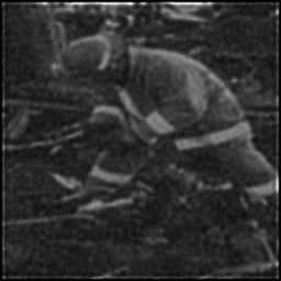
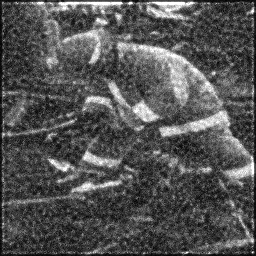
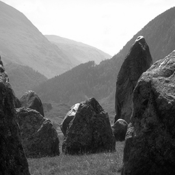
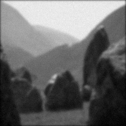
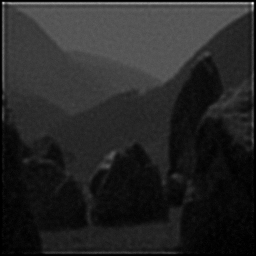
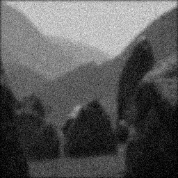
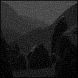
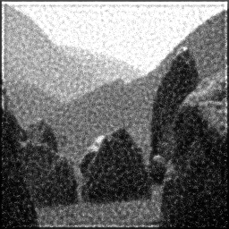
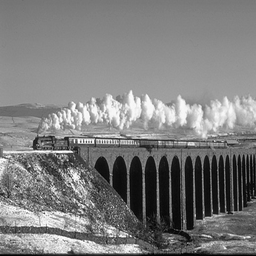
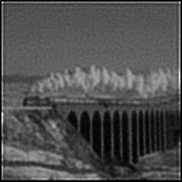
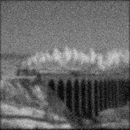
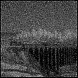
Reconstruction Gallery — 4 Scenes × 3 Scenarios
Method: CPU_baseline | Mismatch: nominal (nominal=True, perturbed=False)

Ground Truth

Measurement
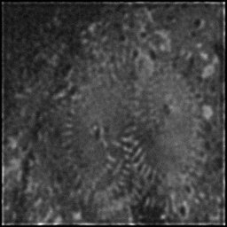
Reconstruction
Ground Truth
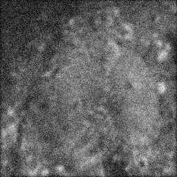
Measurement
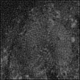
Reconstruction
Ground Truth
Measurement (perturbed)
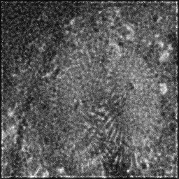
Reconstruction


Mean PSNR Across All Scenes
Per-scene PSNR breakdown (4 scenes)
| Scene | I (PSNR) | I (SSIM) | II (PSNR) | II (SSIM) | III (PSNR) | III (SSIM) |
|---|---|---|---|---|---|---|
| scene_00 | 17.022206064497794 | 0.38380508849556166 | 14.93801985037615 | 0.24399594480247574 | 20.039527108294998 | 0.5012899560940253 |
| scene_01 | 14.231375949985203 | 0.29689664293183293 | 12.92413737908083 | 0.20980780569697918 | 19.225830712320835 | 0.547962131323724 |
| scene_02 | 8.520061941863302 | 0.3871062840596513 | 8.013928482144143 | 0.23077294300010404 | 20.113884181775745 | 0.3416888134023018 |
| scene_03 | 13.297073801541249 | 0.5284335563352818 | 11.66205075678512 | 0.26941399804629346 | 19.61468818224941 | 0.44080752632935544 |
| Mean | 13.267679439471888 | 0.39906039295558193 | 11.884534117096562 | 0.23849767288646312 | 19.748482546160247 | 0.45793710678735156 |
Experimental Setup
Key References
- Axelrod, 'Total internal reflection fluorescence microscopy in cell biology', Traffic 2, 764-774 (2001)
Canonical Datasets
- Cell Tracking Challenge TIRF sequences
- FPbase TIRF imaging examples
Spec DAG — Forward Model Pipeline
C(PSF_TIRF) → D(g, η₃)
Mismatch Parameters
| Symbol | Parameter | Description | Nominal | Perturbed |
|---|---|---|---|---|
| Δθ_i | incidence_angle | Incidence angle error (deg) | 0 | 0.3 |
| Δd | penetration_depth | Penetration depth error (nm) | 0 | 20 |
| Δn | refractive_index | Coverslip refractive index error | 1.515 | 1.52 |
Credits System
Spec Primitives Reference (11 primitives)
Free-space or medium propagation kernel (Fresnel, Rayleigh-Sommerfeld).
Spatial or spatio-temporal amplitude modulation (coded aperture, SLM pattern).
Geometric projection operator (Radon transform, fan-beam, cone-beam).
Sampling in the Fourier / k-space domain (MRI, ptychography).
Shift-invariant convolution with a point-spread function (PSF).
Summation along a physical dimension (spectral, temporal, angular).
Sensor readout with gain g and noise model η (Gaussian, Poisson, mixed).
Patterned illumination (block, Hadamard, random) applied to the scene.
Spectral dispersion element (prism, grating) with shift α and aperture a.
Sample or gantry rotation (CT, electron tomography).
Spectral filter or monochromator selecting a wavelength band.