TEM
Transmission Electron Microscopy
Standard reconstruction benchmark — forward model perfectly known, no calibration needed. Score = 0.5 × clip((PSNR−15)/30, 0, 1) + 0.5 × SSIM
| # | Method | Score | PSNR (dB) | SSIM | Source | |
|---|---|---|---|---|---|---|
| 🥇 |
SwinIR
SwinIR Liang et al., ICCVW 2021
33.4 dB
SSIM 0.930
Checkpoint unavailable
|
0.772 | 33.4 | 0.930 | ✓ Certified | Liang et al., ICCVW 2021 |
| 🥈 |
Noise2Void
Noise2Void Krull et al., CVPR 2019
31.6 dB
SSIM 0.895
Checkpoint unavailable
|
0.724 | 31.6 | 0.895 | ✓ Certified | Krull et al., CVPR 2019 |
| 🥉 | BM3D | 0.635 | 28.5 | 0.820 | ✓ Certified | Dabov et al., IEEE TIP 2007 |
| 4 | Wiener Filter | 0.503 | 24.8 | 0.680 | ✓ Certified | Analytical baseline |
Dataset: PWM Benchmark (4 algorithms)
Blind Reconstruction Challenge — forward model has unknown mismatch, must calibrate from data. Score = 0.4 × PSNR_norm + 0.4 × SSIM + 0.2 × (1 − ‖y − Ĥx̂‖/‖y‖)
| # | Method | Overall Score | Public PSNR / SSIM |
Dev PSNR / SSIM |
Hidden PSNR / SSIM |
Trust | Source |
|---|---|---|---|---|---|---|---|
| 🥇 | SwinIR + gradient | 0.743 |
0.787
32.38 dB / 0.947
|
0.745
30.61 dB / 0.926
|
0.697
27.5 dB / 0.870
|
✓ Certified | Liang et al., ICCVW 2021 |
| 🥈 | BM3D + gradient | 0.626 |
0.677
26.39 dB / 0.843
|
0.620
23.86 dB / 0.764
|
0.580
23.37 dB / 0.745
|
✓ Certified | Dabov et al., IEEE TIP 2007 |
| 🥉 | Noise2Void + gradient | 0.600 |
0.756
30.09 dB / 0.918
|
0.581
22.77 dB / 0.722
|
0.462
18.47 dB / 0.523
|
✓ Certified | Krull et al., CVPR 2019 |
| 4 | Wiener Filter + gradient | 0.576 |
0.582
22.3 dB / 0.703
|
0.579
22.87 dB / 0.726
|
0.566
21.87 dB / 0.684
|
✓ Certified | Analytical baseline |
Complete score requires all 3 tiers (Public + Dev + Hidden).
Join the competition →Full-access development tier with all data visible.
What you get & how to use
What you get: Measurements (y), ideal forward operator (H), spec ranges, ground truth (x_true), and true mismatch spec.
How to use: Load HDF5 → compare reconstruction vs x_true → check consistency → iterate.
What to submit: Reconstructed signals (x_hat) and corrected spec as HDF5.
Public Leaderboard
| # | Method | Score | PSNR | SSIM |
|---|---|---|---|---|
| 1 | SwinIR + gradient | 0.787 | 32.38 | 0.947 |
| 2 | Noise2Void + gradient | 0.756 | 30.09 | 0.918 |
| 3 | BM3D + gradient | 0.677 | 26.39 | 0.843 |
| 4 | Wiener Filter + gradient | 0.582 | 22.3 | 0.703 |
Spec Ranges (3 parameters)
| Parameter | Min | Max | Unit |
|---|---|---|---|
| defocus | -50.0 | 100.0 | nm |
| Cs | -0.01 | 0.02 | mm |
| beam_tilt | -0.5 | 1.0 | mrad |
Blind evaluation tier — no ground truth available.
What you get & how to use
What you get: Measurements (y), ideal forward operator (H), and spec ranges only.
How to use: Apply your pipeline from the Public tier. Use consistency as self-check.
What to submit: Reconstructed signals and corrected spec. Scored server-side.
Dev Leaderboard
| # | Method | Score | PSNR | SSIM |
|---|---|---|---|---|
| 1 | SwinIR + gradient | 0.745 | 30.61 | 0.926 |
| 2 | BM3D + gradient | 0.620 | 23.86 | 0.764 |
| 3 | Noise2Void + gradient | 0.581 | 22.77 | 0.722 |
| 4 | Wiener Filter + gradient | 0.579 | 22.87 | 0.726 |
Spec Ranges (3 parameters)
| Parameter | Min | Max | Unit |
|---|---|---|---|
| defocus | -60.0 | 90.0 | nm |
| Cs | -0.012 | 0.018 | mm |
| beam_tilt | -0.6 | 0.9 | mrad |
Fully blind server-side evaluation — no data download.
What you get & how to use
What you get: No data downloadable. Algorithm runs server-side on hidden measurements.
How to use: Package algorithm as Docker container / Python script. Submit via link.
What to submit: Containerized algorithm accepting y + H, outputting x_hat + corrected spec.
Hidden Leaderboard
| # | Method | Score | PSNR | SSIM |
|---|---|---|---|---|
| 1 | SwinIR + gradient | 0.697 | 27.5 | 0.87 |
| 2 | BM3D + gradient | 0.580 | 23.37 | 0.745 |
| 3 | Wiener Filter + gradient | 0.566 | 21.87 | 0.684 |
| 4 | Noise2Void + gradient | 0.462 | 18.47 | 0.523 |
Spec Ranges (3 parameters)
| Parameter | Min | Max | Unit |
|---|---|---|---|
| defocus | -35.0 | 115.0 | nm |
| Cs | -0.007 | 0.023 | mm |
| beam_tilt | -0.35 | 1.15 | mrad |
Blind Reconstruction Challenge
ChallengeGiven measurements with unknown mismatch and spec ranges (not exact params), reconstruct the original signal. A method must be evaluated on all three tiers for a complete score. Scored on a composite metric: 0.4 × PSNR_norm + 0.4 × SSIM + 0.2 × (1 − ‖y − Ĥx̂‖/‖y‖).
Measurements y, ideal forward model H, spec ranges
Reconstructed signal x̂
About the Imaging Modality
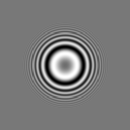
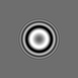
TEM transmits a high-energy electron beam (80-300 keV) through an ultra-thin specimen (<100 nm), magnifying the exit wave with EM lenses. In HRTEM, the image records interference between direct and diffracted beams, convolved by the contrast transfer function (CTF). The CTF introduces oscillating contrast reversals modulated by defocus and spherical aberration. Reconstruction involves CTF correction and, for biological specimens, single-particle averaging.
Principle
Transmission Electron Microscopy transmits a high-energy electron beam (80-300 keV) through an ultra-thin specimen (<100 nm). Electrons interact with the sample via elastic scattering (diffraction contrast, phase contrast) and inelastic scattering (energy loss). The transmitted beam is magnified by electromagnetic lenses to form an image with atomic-level resolution (0.05-0.2 nm in aberration-corrected TEMs).
How to Build the System
Operate a TEM (e.g., JEOL JEM-2100, Thermo Fisher Talos/Titan) under high vacuum (< 10⁻⁵ Pa). Prepare ultra-thin specimens using ultramicrotomy (biological), focused ion beam (FIB) milling (materials), or electropolishing (metals). Load samples on 3 mm TEM grids (Cu or Mo). Align the beam, correct condenser and objective astigmatism, and set appropriate defocus for phase contrast imaging. Use direct-electron detectors for highest DQE.
Common Reconstruction Algorithms
- CTF correction (Contrast Transfer Function for phase contrast imaging)
- Single-particle analysis (cryo-EM: classification, 3-D reconstruction)
- Selected-area electron diffraction (SAED) pattern analysis
- HRTEM image simulation (multislice or Bloch wave)
- Deep-learning denoising for low-dose cryo-EM (Topaz, Warp, cryoSPARC)
Common Mistakes
- Specimen too thick, causing multiple scattering and loss of interpretable contrast
- Beam damage to organic or beam-sensitive materials from excessive electron dose
- Astigmatism and coma not corrected, degrading high-resolution images
- Not accounting for CTF effects when interpreting HRTEM images
- Contamination building up on the specimen under the beam (hydrocarbon deposition)
How to Avoid Mistakes
- Prepare specimens to <50 nm thickness; verify with EELS log-ratio thickness mapping
- Use low-dose protocols and cryo-cooling for beam-sensitive specimens
- Perform careful alignment including Zemlin tableau for Cs-corrected instruments
- Simulate TEM images with known structure and compare; always correct CTF in analysis
- Plasma-clean grids and specimens before loading; use a cryo-shield during imaging
Forward-Model Mismatch Cases
- The widefield fallback produces real-valued output, but TEM forms images from coherent electron wave transmission — the complex-valued exit wave (amplitude and phase from elastic scattering) is lost, destroying quantitative phase-contrast information
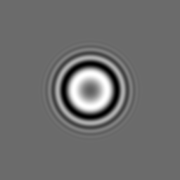
- TEM image contrast arises from coherent interference of scattered electron waves modulated by the contrast transfer function (CTF) — the widefield intensity-based Gaussian blur cannot model the oscillating CTF that produces Thon rings
How to Correct the Mismatch
- Use the TEM operator that models coherent electron imaging: exit wave convolved with the CTF (including defocus, spherical aberration Cs, partial coherence) producing complex-valued image wave
- Reconstruct phase and amplitude using CTF correction (Wiener filtering in Fourier space), or through-focus series exit-wave reconstruction for aberration-corrected quantitative HRTEM
Experimental Setup — Signal Chain

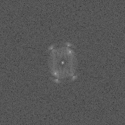
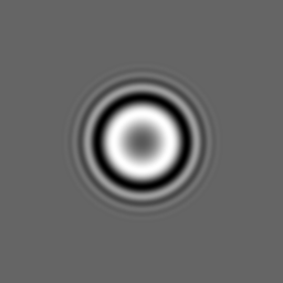
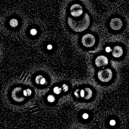
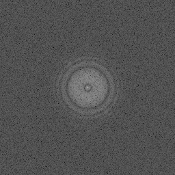
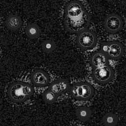
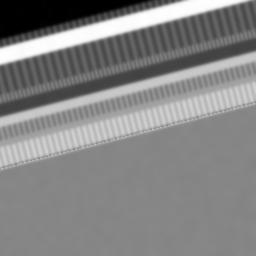
Reconstruction Gallery — 4 Scenes × 3 Scenarios
Method: CPU_baseline | Mismatch: nominal (nominal=True, perturbed=False)
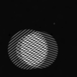
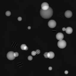
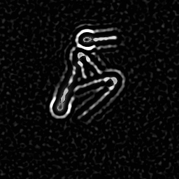
Ground Truth
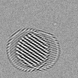
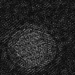
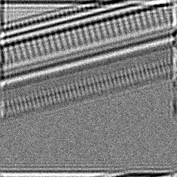
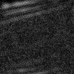
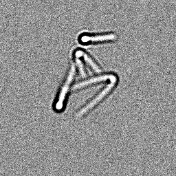
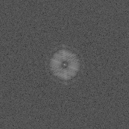
Measurement
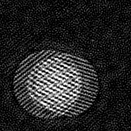
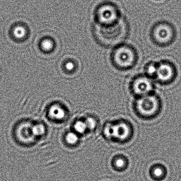
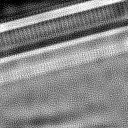
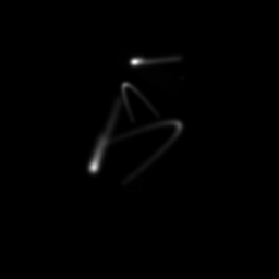
Reconstruction
Ground Truth
Measurement
Reconstruction
Ground Truth
Measurement (perturbed)
Reconstruction

Mean PSNR Across All Scenes
Per-scene PSNR breakdown (4 scenes)
| Scene | I (PSNR) | I (SSIM) | II (PSNR) | II (SSIM) | III (PSNR) | III (SSIM) |
|---|---|---|---|---|---|---|
| scene_00 | 19.6324207258083 | 0.31527741987919805 | 9.246205156285326 | 0.12812342449093475 | 14.964860750841012 | 0.0996307681959596 |
| scene_01 | 17.046641613038403 | 0.2054562168813296 | 7.737947034909802 | 0.17742781554132706 | 17.901544865981993 | 0.2570436605330909 |
| scene_02 | 18.00050936278776 | 0.22798925959780922 | 12.475377438796018 | 0.4694518769608879 | 7.304266436813394 | 0.03589213908786825 |
| scene_03 | 17.231917297353117 | 0.1247969369380569 | 7.096481828254007 | 0.0013938728390127835 | 18.113950160255705 | 0.12117367529267824 |
| Mean | 17.977872249746895 | 0.21837995832409846 | 9.139002864561288 | 0.19409924745804064 | 14.571155553473025 | 0.12843506077739925 |
Experimental Setup
Key References
- Williams & Carter, 'Transmission Electron Microscopy', Springer (2009)
- Haider et al., 'Electron microscopy image enhanced', Nature 392, 768 (1998)
Canonical Datasets
- EMPIAR (Electron Microscopy Public Image Archive)
- NCEM atomic-resolution HRTEM benchmarks
Spec DAG — Forward Model Pipeline
P(e⁻) → C(CTF) → D(g, η₁)
Mismatch Parameters
| Symbol | Parameter | Description | Nominal | Perturbed |
|---|---|---|---|---|
| Δf | defocus | Defocus error (nm) | 0 | 50 |
| ΔC_s | Cs | Spherical aberration error (mm) | 0 | 0.01 |
| Δθ | beam_tilt | Beam tilt error (mrad) | 0 | 0.5 |
Credits System
Spec Primitives Reference (11 primitives)
Free-space or medium propagation kernel (Fresnel, Rayleigh-Sommerfeld).
Spatial or spatio-temporal amplitude modulation (coded aperture, SLM pattern).
Geometric projection operator (Radon transform, fan-beam, cone-beam).
Sampling in the Fourier / k-space domain (MRI, ptychography).
Shift-invariant convolution with a point-spread function (PSF).
Summation along a physical dimension (spectral, temporal, angular).
Sensor readout with gain g and noise model η (Gaussian, Poisson, mixed).
Patterned illumination (block, Hadamard, random) applied to the scene.
Spectral dispersion element (prism, grating) with shift α and aperture a.
Sample or gantry rotation (CT, electron tomography).
Spectral filter or monochromator selecting a wavelength band.