Structured Light
Structured-Light Depth Camera
Standard reconstruction benchmark — forward model perfectly known, no calibration needed. Score = 0.5 × clip((PSNR−15)/30, 0, 1) + 0.5 × SSIM
| # | Method | Score | PSNR (dB) | SSIM | Source | |
|---|---|---|---|---|---|---|
| 🥇 |
PhaseFormer
PhaseFormer Fringe pattern transformer, 2024
34.25 dB
SSIM 0.963
Checkpoint unavailable
|
0.802 | 34.25 | 0.963 | ✓ Certified | Fringe pattern transformer, 2024 |
| 🥈 |
FPP-Net
FPP-Net Feng et al., Opt. Lasers Eng. 2019
33.13 dB
SSIM 0.954
Checkpoint unavailable
|
0.779 | 33.13 | 0.954 | ✓ Certified | Feng et al., Opt. Lasers Eng. 2019 |
| 🥉 | Gray Code | 0.591 | 25.72 | 0.824 | ✓ Certified | Inokuchi et al., Appl. Opt. 1984 |
| 4 | Phase Shifting | 0.564 | 24.87 | 0.798 | ✓ Certified | Srinivasan et al., Appl. Opt. 1984 |
Dataset: PWM Benchmark (4 algorithms)
Blind Reconstruction Challenge — forward model has unknown mismatch, must calibrate from data. Score = 0.4 × PSNR_norm + 0.4 × SSIM + 0.2 × (1 − ‖y − Ĥx̂‖/‖y‖)
| # | Method | Overall Score | Public PSNR / SSIM |
Dev PSNR / SSIM |
Hidden PSNR / SSIM |
Trust | Source |
|---|---|---|---|---|---|---|---|
| 🥇 | PhaseFormer + gradient | 0.726 |
0.795
32.67 dB / 0.950
|
0.717
29.14 dB / 0.903
|
0.667
25.9 dB / 0.829
|
✓ Certified | Fringe pattern transformer, 2024 |
| 🥈 | FPP-Net + gradient | 0.681 |
0.760
31.35 dB / 0.935
|
0.653
25.44 dB / 0.816
|
0.630
25.22 dB / 0.809
|
✓ Certified | Feng et al., Opt. Lasers Eng. 2019 |
| 🥉 | Gray Code + gradient | 0.599 |
0.637
23.98 dB / 0.768
|
0.580
22.45 dB / 0.709
|
0.580
22.38 dB / 0.706
|
✓ Certified | Inokuchi et al., Appl. Opt. 1984 |
| 4 | Phase Shifting + gradient | 0.578 |
0.617
23.25 dB / 0.741
|
0.588
22.89 dB / 0.727
|
0.530
20.52 dB / 0.623
|
✓ Certified | Srinivasan et al., Appl. Opt. 1984 |
Complete score requires all 3 tiers (Public + Dev + Hidden).
Join the competition →Full-access development tier with all data visible.
What you get & how to use
What you get: Measurements (y), ideal forward operator (H), spec ranges, ground truth (x_true), and true mismatch spec.
How to use: Load HDF5 → compare reconstruction vs x_true → check consistency → iterate.
What to submit: Reconstructed signals (x_hat) and corrected spec as HDF5.
Public Leaderboard
| # | Method | Score | PSNR | SSIM |
|---|---|---|---|---|
| 1 | PhaseFormer + gradient | 0.795 | 32.67 | 0.95 |
| 2 | FPP-Net + gradient | 0.760 | 31.35 | 0.935 |
| 3 | Gray Code + gradient | 0.637 | 23.98 | 0.768 |
| 4 | Phase Shifting + gradient | 0.617 | 23.25 | 0.741 |
Spec Ranges (3 parameters)
| Parameter | Min | Max | Unit |
|---|---|---|---|
| baseline | -0.5 | 1.0 | mm |
| pattern_distortion | -1.0 | 2.0 | % |
| ambient_ir | -3.0 | 6.0 | % |
Blind evaluation tier — no ground truth available.
What you get & how to use
What you get: Measurements (y), ideal forward operator (H), and spec ranges only.
How to use: Apply your pipeline from the Public tier. Use consistency as self-check.
What to submit: Reconstructed signals and corrected spec. Scored server-side.
Dev Leaderboard
| # | Method | Score | PSNR | SSIM |
|---|---|---|---|---|
| 1 | PhaseFormer + gradient | 0.717 | 29.14 | 0.903 |
| 2 | FPP-Net + gradient | 0.653 | 25.44 | 0.816 |
| 3 | Phase Shifting + gradient | 0.588 | 22.89 | 0.727 |
| 4 | Gray Code + gradient | 0.580 | 22.45 | 0.709 |
Spec Ranges (3 parameters)
| Parameter | Min | Max | Unit |
|---|---|---|---|
| baseline | -0.6 | 0.9 | mm |
| pattern_distortion | -1.2 | 1.8 | % |
| ambient_ir | -3.6 | 5.4 | % |
Fully blind server-side evaluation — no data download.
What you get & how to use
What you get: No data downloadable. Algorithm runs server-side on hidden measurements.
How to use: Package algorithm as Docker container / Python script. Submit via link.
What to submit: Containerized algorithm accepting y + H, outputting x_hat + corrected spec.
Hidden Leaderboard
| # | Method | Score | PSNR | SSIM |
|---|---|---|---|---|
| 1 | PhaseFormer + gradient | 0.667 | 25.9 | 0.829 |
| 2 | FPP-Net + gradient | 0.630 | 25.22 | 0.809 |
| 3 | Gray Code + gradient | 0.580 | 22.38 | 0.706 |
| 4 | Phase Shifting + gradient | 0.530 | 20.52 | 0.623 |
Spec Ranges (3 parameters)
| Parameter | Min | Max | Unit |
|---|---|---|---|
| baseline | -0.35 | 1.15 | mm |
| pattern_distortion | -0.7 | 2.3 | % |
| ambient_ir | -2.1 | 6.9 | % |
Blind Reconstruction Challenge
ChallengeGiven measurements with unknown mismatch and spec ranges (not exact params), reconstruct the original signal. A method must be evaluated on all three tiers for a complete score. Scored on a composite metric: 0.4 × PSNR_norm + 0.4 × SSIM + 0.2 × (1 − ‖y − Ĥx̂‖/‖y‖).
Measurements y, ideal forward model H, spec ranges
Reconstructed signal x̂
About the Imaging Modality
Structured-light depth cameras project a known pattern (IR dot pattern, fringe, or binary code) onto the scene and infer depth from the pattern deformation observed by a camera offset from the projector. For coded structured light (e.g., Kinect v1), depth is computed via triangulation from the correspondence between projected and observed pattern features. For phase-shifting methods, multiple fringe patterns encode depth as the local phase. Primary challenges include occlusion in the projector-camera baseline, ambient light interference, and depth discontinuity errors.
Principle
Structured-light depth sensing projects a known pattern (stripes, dots, coded binary patterns) onto the scene and observes the pattern deformation with a camera from a different viewpoint. The displacement (disparity) of each pattern element between projected and observed positions encodes the surface depth via triangulation. Dense depth maps are obtained by identifying pattern correspondences across the scene.
How to Build the System
Arrange a projector (DLP or laser dot projector) and camera with a known baseline separation (5-25 cm) and convergent geometry. Calibrate the projector-camera system (intrinsics and extrinsics) using a planar calibration target. For temporal coding (Gray code), project multiple patterns sequentially. For spatial coding (single-shot, e.g., Apple FaceID dot projector), use a diffractive optical element to generate a unique dot pattern.
Common Reconstruction Algorithms
- Gray code + phase shifting (sequential multi-pattern decoding)
- Single-shot coded pattern matching (speckle or pseudo-random dot decoding)
- Phase unwrapping for sinusoidal fringe projection
- Stereo matching applied to textured scenes (active stereo)
- Deep-learning depth estimation from structured-light patterns
Common Mistakes
- Ambient light washing out the projected pattern, losing depth information
- Specular (shiny) surfaces reflecting the projector into the camera, causing erroneous depth
- Occlusion zones where the projector illuminates but the camera cannot see (shadowed regions)
- Insufficient projector resolution limiting the achievable depth precision
- Color/reflectance variations in the scene altering perceived pattern intensity
How to Avoid Mistakes
- Use NIR projector + camera with ambient-light rejection filter
- Apply polarization filtering or spray surfaces with matte coating for calibration
- Add a second camera or projector to reduce occlusion zones
- Use high-resolution projectors (1080p+) and fine patterns for sub-mm precision
- Use binary or phase-shifting patterns that are robust to reflectance variations
Forward-Model Mismatch Cases
- The widefield fallback applies spatial blur, but structured-light depth sensing projects known patterns and measures their deformation via triangulation — the depth-encoding pattern correspondence between projector and camera is absent
- Structured light extracts depth from disparity between projected and observed pattern positions (d = f*B/disparity) — the widefield blur produces no disparity information and cannot encode surface depth
How to Correct the Mismatch
- Use the structured-light operator that models pattern projection (Gray code, sinusoidal fringe, or speckle) and camera observation from a different viewpoint: depth is encoded in pattern deformation due to surface geometry
- Extract depth maps using pattern decoding (Gray code → correspondence → triangulation) or phase unwrapping (sinusoidal fringe → depth) with calibrated projector-camera geometry
Experimental Setup — Signal Chain

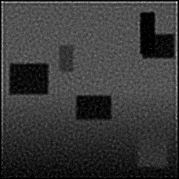
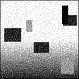
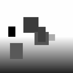
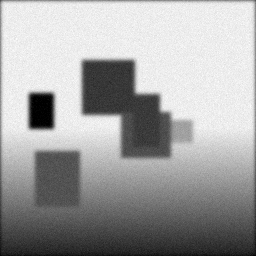
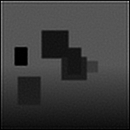
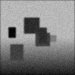
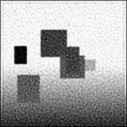
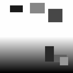
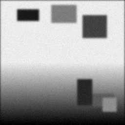
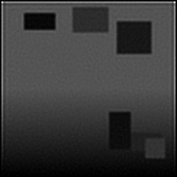
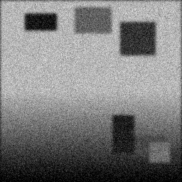
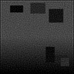
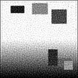
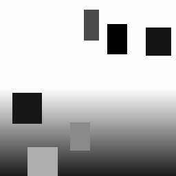
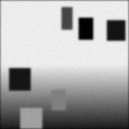
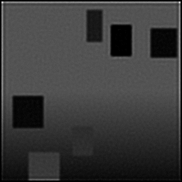
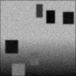
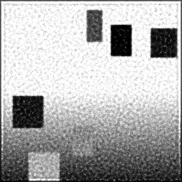
Reconstruction Gallery — 4 Scenes × 3 Scenarios
Method: CPU_baseline | Mismatch: nominal (nominal=True, perturbed=False)
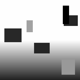
Ground Truth
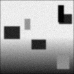
Measurement
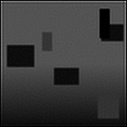
Reconstruction
Ground Truth
Measurement
Reconstruction
Ground Truth
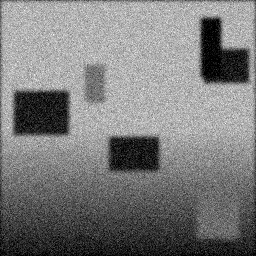
Measurement (perturbed)
Reconstruction


Mean PSNR Across All Scenes
Per-scene PSNR breakdown (4 scenes)
| Scene | I (PSNR) | I (SSIM) | II (PSNR) | II (SSIM) | III (PSNR) | III (SSIM) |
|---|---|---|---|---|---|---|
| scene_00 | 5.527214497768322 | 0.4672006439363062 | 5.459345679167983 | 0.19945611529107565 | 18.401943105213206 | 0.2341331320438871 |
| scene_01 | 5.806026384875609 | 0.4796046249826327 | 6.030423203911414 | 0.19344004863131214 | 18.47044552189445 | 0.22669922821491817 |
| scene_02 | 5.6571772261462066 | 0.46600075432368365 | 5.076086325487175 | 0.20923461502441765 | 18.605513677538003 | 0.23724583293967508 |
| scene_03 | 5.389777474892018 | 0.468956853362985 | 5.2322280218118955 | 0.2040550582761015 | 18.40005847928955 | 0.2386520108290784 |
| Mean | 5.595048895920539 | 0.47044071915140184 | 5.449520807594617 | 0.20154645930572673 | 18.469490195983802 | 0.23418255100688967 |
Experimental Setup
Key References
- Geng, 'Structured-light 3D surface imaging: a tutorial', Advances in Optics and Photonics 3, 128-160 (2011)
Canonical Datasets
- Middlebury stereo benchmark
- ETH3D multi-view stereo benchmark
Spec DAG — Forward Model Pipeline
S(pattern) → Π(triangulation) → D(g, η₁)
Mismatch Parameters
| Symbol | Parameter | Description | Nominal | Perturbed |
|---|---|---|---|---|
| Δb | baseline | Projector-camera baseline error (mm) | 0 | 0.5 |
| ΔP | pattern_distortion | Pattern distortion (%) | 0 | 1.0 |
| I_amb | ambient_ir | Ambient IR interference (%) | 0 | 3.0 |
Credits System
Spec Primitives Reference (11 primitives)
Free-space or medium propagation kernel (Fresnel, Rayleigh-Sommerfeld).
Spatial or spatio-temporal amplitude modulation (coded aperture, SLM pattern).
Geometric projection operator (Radon transform, fan-beam, cone-beam).
Sampling in the Fourier / k-space domain (MRI, ptychography).
Shift-invariant convolution with a point-spread function (PSF).
Summation along a physical dimension (spectral, temporal, angular).
Sensor readout with gain g and noise model η (Gaussian, Poisson, mixed).
Patterned illumination (block, Hadamard, random) applied to the scene.
Spectral dispersion element (prism, grating) with shift α and aperture a.
Sample or gantry rotation (CT, electron tomography).
Spectral filter or monochromator selecting a wavelength band.