STEM
Scanning TEM
Standard reconstruction benchmark — forward model perfectly known, no calibration needed. Score = 0.5 × clip((PSNR−15)/30, 0, 1) + 0.5 × SSIM
| # | Method | Score | PSNR (dB) | SSIM | Source | |
|---|---|---|---|---|---|---|
| 🥇 |
SwinIR
SwinIR Liang et al., ICCVW 2021
33.4 dB
SSIM 0.930
Checkpoint unavailable
|
0.772 | 33.4 | 0.930 | ✓ Certified | Liang et al., ICCVW 2021 |
| 🥈 |
Noise2Void
Noise2Void Krull et al., CVPR 2019
31.6 dB
SSIM 0.895
Checkpoint unavailable
|
0.724 | 31.6 | 0.895 | ✓ Certified | Krull et al., CVPR 2019 |
| 🥉 | BM3D | 0.635 | 28.5 | 0.820 | ✓ Certified | Dabov et al., IEEE TIP 2007 |
| 4 | Wiener Filter | 0.503 | 24.8 | 0.680 | ✓ Certified | Analytical baseline |
Dataset: PWM Benchmark (4 algorithms)
Blind Reconstruction Challenge — forward model has unknown mismatch, must calibrate from data. Score = 0.4 × PSNR_norm + 0.4 × SSIM + 0.2 × (1 − ‖y − Ĥx̂‖/‖y‖)
| # | Method | Overall Score | Public PSNR / SSIM |
Dev PSNR / SSIM |
Hidden PSNR / SSIM |
Trust | Source |
|---|---|---|---|---|---|---|---|
| 🥇 | SwinIR + gradient | 0.683 |
0.761
31.18 dB / 0.933
|
0.700
27.95 dB / 0.880
|
0.589
23.03 dB / 0.732
|
✓ Certified | Liang et al., ICCVW 2021 |
| 🥈 | BM3D + gradient | 0.649 |
0.673
26.19 dB / 0.837
|
0.661
25.89 dB / 0.829
|
0.614
24.26 dB / 0.778
|
✓ Certified | Dabov et al., IEEE TIP 2007 |
| 🥉 | Noise2Void + gradient | 0.601 |
0.754
29.96 dB / 0.916
|
0.562
22.29 dB / 0.702
|
0.486
19.35 dB / 0.567
|
✓ Certified | Krull et al., CVPR 2019 |
| 4 | Wiener Filter + gradient | 0.536 |
0.586
22.46 dB / 0.709
|
0.534
20.7 dB / 0.632
|
0.489
19.93 dB / 0.595
|
✓ Certified | Analytical baseline |
Complete score requires all 3 tiers (Public + Dev + Hidden).
Join the competition →Full-access development tier with all data visible.
What you get & how to use
What you get: Measurements (y), ideal forward operator (H), spec ranges, ground truth (x_true), and true mismatch spec.
How to use: Load HDF5 → compare reconstruction vs x_true → check consistency → iterate.
What to submit: Reconstructed signals (x_hat) and corrected spec as HDF5.
Public Leaderboard
| # | Method | Score | PSNR | SSIM |
|---|---|---|---|---|
| 1 | SwinIR + gradient | 0.761 | 31.18 | 0.933 |
| 2 | Noise2Void + gradient | 0.754 | 29.96 | 0.916 |
| 3 | BM3D + gradient | 0.673 | 26.19 | 0.837 |
| 4 | Wiener Filter + gradient | 0.586 | 22.46 | 0.709 |
Spec Ranges (3 parameters)
| Parameter | Min | Max | Unit |
|---|---|---|---|
| probe_size | -0.1 | 0.2 | Å |
| convergence_angle | -0.5 | 1.0 | mrad |
| scan_distortion | -0.5 | 1.0 | % |
Blind evaluation tier — no ground truth available.
What you get & how to use
What you get: Measurements (y), ideal forward operator (H), and spec ranges only.
How to use: Apply your pipeline from the Public tier. Use consistency as self-check.
What to submit: Reconstructed signals and corrected spec. Scored server-side.
Dev Leaderboard
| # | Method | Score | PSNR | SSIM |
|---|---|---|---|---|
| 1 | SwinIR + gradient | 0.700 | 27.95 | 0.88 |
| 2 | BM3D + gradient | 0.661 | 25.89 | 0.829 |
| 3 | Noise2Void + gradient | 0.562 | 22.29 | 0.702 |
| 4 | Wiener Filter + gradient | 0.534 | 20.7 | 0.632 |
Spec Ranges (3 parameters)
| Parameter | Min | Max | Unit |
|---|---|---|---|
| probe_size | -0.12 | 0.18 | Å |
| convergence_angle | -0.6 | 0.9 | mrad |
| scan_distortion | -0.6 | 0.9 | % |
Fully blind server-side evaluation — no data download.
What you get & how to use
What you get: No data downloadable. Algorithm runs server-side on hidden measurements.
How to use: Package algorithm as Docker container / Python script. Submit via link.
What to submit: Containerized algorithm accepting y + H, outputting x_hat + corrected spec.
Hidden Leaderboard
| # | Method | Score | PSNR | SSIM |
|---|---|---|---|---|
| 1 | BM3D + gradient | 0.614 | 24.26 | 0.778 |
| 2 | SwinIR + gradient | 0.589 | 23.03 | 0.732 |
| 3 | Wiener Filter + gradient | 0.489 | 19.93 | 0.595 |
| 4 | Noise2Void + gradient | 0.486 | 19.35 | 0.567 |
Spec Ranges (3 parameters)
| Parameter | Min | Max | Unit |
|---|---|---|---|
| probe_size | -0.07 | 0.23 | Å |
| convergence_angle | -0.35 | 1.15 | mrad |
| scan_distortion | -0.35 | 1.15 | % |
Blind Reconstruction Challenge
ChallengeGiven measurements with unknown mismatch and spec ranges (not exact params), reconstruct the original signal. A method must be evaluated on all three tiers for a complete score. Scored on a composite metric: 0.4 × PSNR_norm + 0.4 × SSIM + 0.2 × (1 − ‖y − Ĥx̂‖/‖y‖).
Measurements y, ideal forward model H, spec ranges
Reconstructed signal x̂
About the Imaging Modality
STEM focuses the electron beam to a sub-angstrom probe and scans it across a thin specimen. The HAADF detector collects electrons scattered to large angles (>50 mrad), producing incoherent Z-contrast images where intensity scales as ~Z^1.7, enabling direct compositional interpretation at atomic resolution. Aberration correction (C3/C5 correctors) achieves sub-50 pm probe sizes. Primary degradations include scan distortion, probe instability, and radiation damage.
Principle
Scanning TEM focuses the electron beam to a fine probe (0.05-1 nm) and scans it across the specimen. Multiple detectors collect signals simultaneously: bright-field (BF), annular dark-field (ADF), and high-angle annular dark-field (HAADF). HAADF-STEM provides Z-contrast imaging where intensity scales approximately as Z^1.7, enabling direct interpretation of atomic columns by atomic number.
How to Build the System
Use an aberration-corrected STEM (probe-corrected, e.g., Thermo Fisher Titan Themis or JEOL ARM300F). Align the probe-corrector to minimize C₃ and C₅ aberrations, achieving sub-Ångström probe size. Adjust camera length for HAADF inner angle (typically 50-80 mrad for Z-contrast). Prepare atomically thin specimens by FIB or mechanical exfoliation. Use drift-corrected frame integration for high-quality atomic-resolution images.
Common Reconstruction Algorithms
- Atom column detection and quantification (peak finding, Gaussian fitting)
- Strain mapping via geometric phase analysis (GPA) or peak-pair analysis
- Multi-frame averaging with rigid/non-rigid registration for noise reduction
- HAADF simulation (frozen-phonon multislice) for quantitative comparison
- Deep-learning STEM image denoising and super-resolution
Common Mistakes
- Probe aberrations not fully corrected, producing probe tails and delocalization
- Scan distortion (flyback, drift) causing apparent lattice strain artifacts
- Sample mistilt from zone axis, reducing contrast of atomic columns
- Amorphous surface layers (from FIB damage) obscuring atomic contrast
- Electron channeling effects complicating quantitative HAADF interpretation
How to Avoid Mistakes
- Tune corrector regularly using Zemlin tableau or Ronchigram analysis
- Apply scan distortion correction using known lattice spacings as reference
- Tilt to exact zone axis using CBED pattern or Ronchigram fine alignment
- Use low-kV FIB final polishing or Ar-ion milling to minimize surface damage
- Simulate HAADF images with the exact specimen thickness for quantitative analysis
Forward-Model Mismatch Cases
- The widefield fallback applies a Gaussian PSF blur, but STEM forms images by rastering a focused electron probe (~0.1 nm) and collecting scattered electrons with annular detectors — the contrast depends on detector geometry (BF, ADF, HAADF) not optical PSF shape
- HAADF-STEM contrast is proportional to Z^~1.7 (atomic number contrast), enabling direct chemical imaging — the widefield PSF convolution produces optical-type blur with no Z-contrast information
How to Correct the Mismatch
- Use the STEM operator that models the electron probe profile (aberration-corrected sub-angstrom) and detector-dependent signal collection: ADF integrates scattered electrons over the annular detector range
- For quantitative STEM, include the probe-forming aberration function, thermal diffuse scattering, and detector inner/outer angle to correctly model Z-contrast and strain mapping
Experimental Setup — Signal Chain

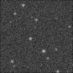
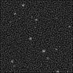
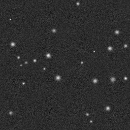
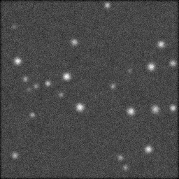
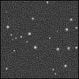
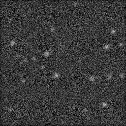
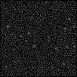
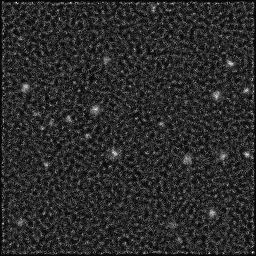
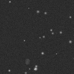
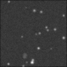
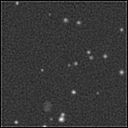
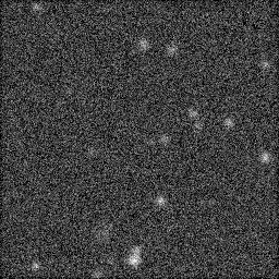
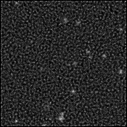
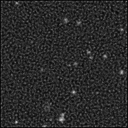
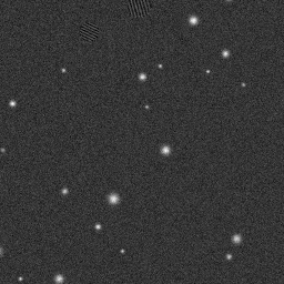
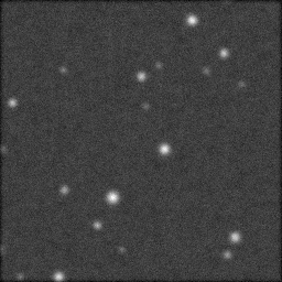
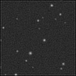
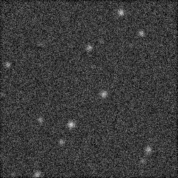
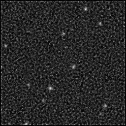
Reconstruction Gallery — 4 Scenes × 3 Scenarios
Method: CPU_baseline | Mismatch: nominal (nominal=True, perturbed=False)
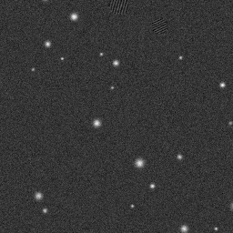
Ground Truth
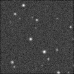
Measurement
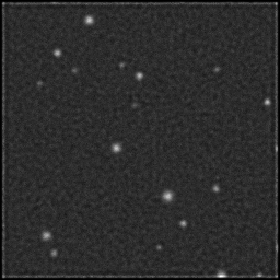
Reconstruction
Ground Truth
Measurement
Reconstruction
Ground Truth
Measurement (perturbed)
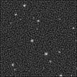
Reconstruction
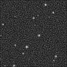
Mean PSNR Across All Scenes
Per-scene PSNR breakdown (4 scenes)
| Scene | I (PSNR) | I (SSIM) | II (PSNR) | II (SSIM) | III (PSNR) | III (SSIM) |
|---|---|---|---|---|---|---|
| scene_00 | 23.51322858456625 | 0.3680334261076263 | 18.321872109157592 | 0.10385815436617447 | 20.03444592103245 | 0.1989493017944018 |
| scene_01 | 20.039820761387634 | 0.29166542696823705 | 18.85922982415404 | 0.12798625129650684 | 20.031642094176974 | 0.19752602173448866 |
| scene_02 | 23.283012767044198 | 0.357495155445897 | 18.4465452279848 | 0.09369496983474383 | 20.2796683331393 | 0.18597290071365627 |
| scene_03 | 23.31589368033676 | 0.36687406178777526 | 18.405990402819242 | 0.10758808193384366 | 20.100674151892584 | 0.20008535528637864 |
| Mean | 22.53798894833371 | 0.3460170175773839 | 18.50840939102892 | 0.10828186435781721 | 20.111607625060326 | 0.19563339488223133 |
Experimental Setup
Key References
- Pennycook & Nellist, 'Z-Contrast STEM Imaging', Springer (2011)
- Krivanek et al., 'Atom-by-atom structural and chemical analysis by annular dark-field electron microscopy', Nature 464, 571 (2010)
Canonical Datasets
- NCEM Molecular Foundry STEM benchmarks
- EMPIAR STEM datasets
Spec DAG — Forward Model Pipeline
P(e⁻) → C(probe) → D(g, η₁)
Mismatch Parameters
| Symbol | Parameter | Description | Nominal | Perturbed |
|---|---|---|---|---|
| Δd_p | probe_size | Probe size error (Å) | 0 | 0.1 |
| Δα | convergence_angle | Convergence semi-angle error (mrad) | 0 | 0.5 |
| Δs | scan_distortion | Scan distortion (%) | 0 | 0.5 |
Credits System
Spec Primitives Reference (11 primitives)
Free-space or medium propagation kernel (Fresnel, Rayleigh-Sommerfeld).
Spatial or spatio-temporal amplitude modulation (coded aperture, SLM pattern).
Geometric projection operator (Radon transform, fan-beam, cone-beam).
Sampling in the Fourier / k-space domain (MRI, ptychography).
Shift-invariant convolution with a point-spread function (PSF).
Summation along a physical dimension (spectral, temporal, angular).
Sensor readout with gain g and noise model η (Gaussian, Poisson, mixed).
Patterned illumination (block, Hadamard, random) applied to the scene.
Spectral dispersion element (prism, grating) with shift α and aperture a.
Sample or gantry rotation (CT, electron tomography).
Spectral filter or monochromator selecting a wavelength band.