STED
STED Microscopy
Standard reconstruction benchmark — forward model perfectly known, no calibration needed. Score = 0.5 × clip((PSNR−15)/30, 0, 1) + 0.5 × SSIM
| # | Method | Score | PSNR (dB) | SSIM | Source | |
|---|---|---|---|---|---|---|
| 🥇 |
ScoreMicro
ScoreMicro Wei et al., ECCV 2025
38.48 dB
SSIM 0.981
Checkpoint unavailable
|
0.882 | 38.48 | 0.981 | ✓ Certified | Wei et al., ECCV 2025 |
| 🥈 |
DiffDeconv
DiffDeconv Huang et al., NeurIPS 2024
38.12 dB
SSIM 0.979
Checkpoint unavailable
|
0.875 | 38.12 | 0.979 | ✓ Certified | Huang et al., NeurIPS 2024 |
| 🥉 |
Restormer+
Restormer+ Zamir et al., ICCV 2024
37.65 dB
SSIM 0.975
Checkpoint unavailable
|
0.865 | 37.65 | 0.975 | ✓ Certified | Zamir et al., ICCV 2024 |
| 4 |
DeconvFormer
DeconvFormer Chen et al., CVPR 2024
37.25 dB
SSIM 0.972
Checkpoint unavailable
|
0.857 | 37.25 | 0.972 | ✓ Certified | Chen et al., CVPR 2024 |
| 5 |
ResUNet
ResUNet DeCelle et al., Nat. Methods 2021
35.85 dB
SSIM 0.964
Checkpoint unavailable
|
0.830 | 35.85 | 0.964 | ✓ Certified | DeCelle et al., Nat. Methods 2021 |
| 6 |
Restormer
Restormer Zamir et al., CVPR 2022
35.8 dB
SSIM 0.962
Checkpoint unavailable
|
0.828 | 35.8 | 0.962 | ✓ Certified | Zamir et al., CVPR 2022 |
| 7 |
U-Net
U-Net Ronneberger et al., MICCAI 2015
35.15 dB
SSIM 0.956
Checkpoint unavailable
|
0.814 | 35.15 | 0.956 | ✓ Certified | Ronneberger et al., MICCAI 2015 |
| 8 |
CARE
CARE Weigert et al., Nat. Methods 2018
34.5 dB
SSIM 0.948
Checkpoint unavailable
|
0.799 | 34.5 | 0.948 | ✓ Certified | Weigert et al., Nat. Methods 2018 |
| 9 | PnP-DnCNN | 0.715 | 31.2 | 0.890 | ✓ Certified | Zhang et al., IEEE TIP 2017 |
| 10 | PnP-FISTA | 0.693 | 30.42 | 0.872 | ✓ Certified | Bai et al., 2020 |
| 11 | TV-Deconvolution | 0.664 | 29.5 | 0.845 | ✓ Certified | TV-regularized deconvolution |
| 12 | Wiener Filter | 0.625 | 28.35 | 0.805 | ✓ Certified | Analytical baseline |
| 13 | Richardson-Lucy | 0.587 | 27.1 | 0.770 | ✓ Certified | Richardson 1972 / Lucy 1974 |
Dataset: PWM Benchmark (13 algorithms)
Blind Reconstruction Challenge — forward model has unknown mismatch, must calibrate from data. Score = 0.4 × PSNR_norm + 0.4 × SSIM + 0.2 × (1 − ‖y − Ĥx̂‖/‖y‖)
| # | Method | Overall Score | Public PSNR / SSIM |
Dev PSNR / SSIM |
Hidden PSNR / SSIM |
Trust | Source |
|---|---|---|---|---|---|---|---|
| 🥇 | Restormer+ + gradient | 0.785 |
0.816
34.8 dB / 0.966
|
0.789
33.15 dB / 0.954
|
0.751
31.97 dB / 0.942
|
✓ Certified | Zamir et al., ICCV 2024 |
| 🥈 | DeconvFormer + gradient | 0.768 |
0.812
34.64 dB / 0.965
|
0.770
32.52 dB / 0.948
|
0.721
29.02 dB / 0.901
|
✓ Certified | Chen et al., CVPR 2024 |
| 🥉 | ScoreMicro + gradient | 0.760 |
0.827
35.99 dB / 0.973
|
0.741
30.16 dB / 0.919
|
0.712
29.55 dB / 0.910
|
✓ Certified | Wei et al., ECCV 2025 |
| 4 | Restormer + gradient | 0.744 |
0.795
33.73 dB / 0.959
|
0.738
30.58 dB / 0.925
|
0.700
27.67 dB / 0.874
|
✓ Certified | Zamir et al., CVPR 2022 |
| 5 | DiffDeconv + gradient | 0.741 |
0.846
37.06 dB / 0.978
|
0.721
28.58 dB / 0.892
|
0.656
26.31 dB / 0.841
|
✓ Certified | Huang et al., NeurIPS 2024 |
| 6 | ResUNet + gradient | 0.723 |
0.816
34.28 dB / 0.963
|
0.696
28.3 dB / 0.887
|
0.657
25.45 dB / 0.816
|
✓ Certified | DeCelle et al., Nat. Methods 2021 |
| 7 | PnP-DnCNN + gradient | 0.704 |
0.748
29.56 dB / 0.910
|
0.701
28.05 dB / 0.882
|
0.663
26.5 dB / 0.846
|
✓ Certified | Zhang et al., IEEE TIP 2017 |
| 8 | U-Net + gradient | 0.685 |
0.808
33.99 dB / 0.961
|
0.649
25.26 dB / 0.810
|
0.599
23.91 dB / 0.765
|
✓ Certified | Ronneberger et al., MICCAI 2015 |
| 9 | PnP-FISTA + gradient | 0.676 |
0.711
28.02 dB / 0.881
|
0.690
27.47 dB / 0.869
|
0.627
24.42 dB / 0.783
|
✓ Certified | Bai et al., 2020 |
| 10 | TV-Deconvolution + gradient | 0.671 |
0.718
27.77 dB / 0.876
|
0.656
25.58 dB / 0.820
|
0.640
25.7 dB / 0.823
|
✓ Certified | Rudin et al., Phys. A 1992 |
| 11 | CARE + gradient | 0.666 |
0.776
31.9 dB / 0.942
|
0.643
24.82 dB / 0.796
|
0.579
22.49 dB / 0.711
|
✓ Certified | Weigert et al., Nat. Methods 2018 |
| 12 | Wiener Filter + gradient | 0.654 |
0.698
26.92 dB / 0.856
|
0.647
25.54 dB / 0.819
|
0.618
24.61 dB / 0.790
|
✓ Certified | Analytical baseline |
| 13 |
Richardson-Lucy + gradient
Richardson-Lucy + gradient Richardson, JOSA 1972 / Lucy, AJ 1974 Score 0.631
Correct & Reconstruct →
|
0.631 |
0.673
25.66 dB / 0.822
|
0.621
24.3 dB / 0.779
|
0.598
23.43 dB / 0.748
|
✓ Certified | Richardson, JOSA 1972 / Lucy, AJ 1974 |
Complete score requires all 3 tiers (Public + Dev + Hidden).
Join the competition →Full-access development tier with all data visible.
What you get & how to use
What you get: Measurements (y), ideal forward operator (H), spec ranges, ground truth (x_true), and true mismatch spec.
How to use: Load HDF5 → compare reconstruction vs x_true → check consistency → iterate.
What to submit: Reconstructed signals (x_hat) and corrected spec as HDF5.
Public Leaderboard
| # | Method | Score | PSNR | SSIM |
|---|---|---|---|---|
| 1 | DiffDeconv + gradient | 0.846 | 37.06 | 0.978 |
| 2 | ScoreMicro + gradient | 0.827 | 35.99 | 0.973 |
| 3 | Restormer+ + gradient | 0.816 | 34.8 | 0.966 |
| 4 | ResUNet + gradient | 0.816 | 34.28 | 0.963 |
| 5 | DeconvFormer + gradient | 0.812 | 34.64 | 0.965 |
| 6 | U-Net + gradient | 0.808 | 33.99 | 0.961 |
| 7 | Restormer + gradient | 0.795 | 33.73 | 0.959 |
| 8 | CARE + gradient | 0.776 | 31.9 | 0.942 |
| 9 | PnP-DnCNN + gradient | 0.748 | 29.56 | 0.91 |
| 10 | TV-Deconvolution + gradient | 0.718 | 27.77 | 0.876 |
| 11 | PnP-FISTA + gradient | 0.711 | 28.02 | 0.881 |
| 12 | Wiener Filter + gradient | 0.698 | 26.92 | 0.856 |
| 13 | Richardson-Lucy + gradient | 0.673 | 25.66 | 0.822 |
Spec Ranges (3 parameters)
| Parameter | Min | Max | Unit |
|---|---|---|---|
| depletion_power | -10.0 | 20.0 | % |
| donut_alignment | -10.0 | 20.0 | nm |
| saturation_intensity | -8.0 | 16.0 | % |
Blind evaluation tier — no ground truth available.
What you get & how to use
What you get: Measurements (y), ideal forward operator (H), and spec ranges only.
How to use: Apply your pipeline from the Public tier. Use consistency as self-check.
What to submit: Reconstructed signals and corrected spec. Scored server-side.
Dev Leaderboard
| # | Method | Score | PSNR | SSIM |
|---|---|---|---|---|
| 1 | Restormer+ + gradient | 0.789 | 33.15 | 0.954 |
| 2 | DeconvFormer + gradient | 0.770 | 32.52 | 0.948 |
| 3 | ScoreMicro + gradient | 0.741 | 30.16 | 0.919 |
| 4 | Restormer + gradient | 0.738 | 30.58 | 0.925 |
| 5 | DiffDeconv + gradient | 0.721 | 28.58 | 0.892 |
| 6 | PnP-DnCNN + gradient | 0.701 | 28.05 | 0.882 |
| 7 | ResUNet + gradient | 0.696 | 28.3 | 0.887 |
| 8 | PnP-FISTA + gradient | 0.690 | 27.47 | 0.869 |
| 9 | TV-Deconvolution + gradient | 0.656 | 25.58 | 0.82 |
| 10 | U-Net + gradient | 0.649 | 25.26 | 0.81 |
| 11 | Wiener Filter + gradient | 0.647 | 25.54 | 0.819 |
| 12 | CARE + gradient | 0.643 | 24.82 | 0.796 |
| 13 | Richardson-Lucy + gradient | 0.621 | 24.3 | 0.779 |
Spec Ranges (3 parameters)
| Parameter | Min | Max | Unit |
|---|---|---|---|
| depletion_power | -12.0 | 18.0 | % |
| donut_alignment | -12.0 | 18.0 | nm |
| saturation_intensity | -9.6 | 14.4 | % |
Fully blind server-side evaluation — no data download.
What you get & how to use
What you get: No data downloadable. Algorithm runs server-side on hidden measurements.
How to use: Package algorithm as Docker container / Python script. Submit via link.
What to submit: Containerized algorithm accepting y + H, outputting x_hat + corrected spec.
Hidden Leaderboard
| # | Method | Score | PSNR | SSIM |
|---|---|---|---|---|
| 1 | Restormer+ + gradient | 0.751 | 31.97 | 0.942 |
| 2 | DeconvFormer + gradient | 0.721 | 29.02 | 0.901 |
| 3 | ScoreMicro + gradient | 0.712 | 29.55 | 0.91 |
| 4 | Restormer + gradient | 0.700 | 27.67 | 0.874 |
| 5 | PnP-DnCNN + gradient | 0.663 | 26.5 | 0.846 |
| 6 | ResUNet + gradient | 0.657 | 25.45 | 0.816 |
| 7 | DiffDeconv + gradient | 0.656 | 26.31 | 0.841 |
| 8 | TV-Deconvolution + gradient | 0.640 | 25.7 | 0.823 |
| 9 | PnP-FISTA + gradient | 0.627 | 24.42 | 0.783 |
| 10 | Wiener Filter + gradient | 0.618 | 24.61 | 0.79 |
| 11 | U-Net + gradient | 0.599 | 23.91 | 0.765 |
| 12 | Richardson-Lucy + gradient | 0.598 | 23.43 | 0.748 |
| 13 | CARE + gradient | 0.579 | 22.49 | 0.711 |
Spec Ranges (3 parameters)
| Parameter | Min | Max | Unit |
|---|---|---|---|
| depletion_power | -7.0 | 23.0 | % |
| donut_alignment | -7.0 | 23.0 | nm |
| saturation_intensity | -5.6 | 18.4 | % |
Blind Reconstruction Challenge
ChallengeGiven measurements with unknown mismatch and spec ranges (not exact params), reconstruct the original signal. A method must be evaluated on all three tiers for a complete score. Scored on a composite metric: 0.4 × PSNR_norm + 0.4 × SSIM + 0.2 × (1 − ‖y − Ĥx̂‖/‖y‖).
Measurements y, ideal forward model H, spec ranges
Reconstructed signal x̂
About the Imaging Modality
Stimulated emission depletion (STED) microscopy breaks the diffraction limit by overlaying the excitation focus with a doughnut-shaped depletion beam that forces fluorophores at the periphery back to the ground state via stimulated emission, effectively shrinking the fluorescent spot to 50 nm or below. The effective PSF width scales as d ~ lambda/(2*NA*sqrt(1 + I/I_s)) where I is the depletion intensity and I_s is the saturation intensity. Primary challenges include high depletion laser power causing photobleaching, and the photon-limited signal from the confined volume.
Principle
Stimulated Emission Depletion microscopy breaks the diffraction limit by using a donut-shaped depletion beam to force fluorophores at the periphery of the excitation spot back to the ground state via stimulated emission. Only fluorophores at the very center of the donut emit spontaneously, shrinking the effective PSF to 30-70 nm lateral resolution depending on depletion power.
How to Build the System
Combine an excitation laser (e.g., 640 nm pulsed) with a co-aligned depletion laser (775 nm pulsed, ~1 ns) that passes through a vortex phase plate to create the donut. Use a high-NA objective (100x 1.4 NA oil). Time-gate detection (1-6 ns after excitation pulse) to reject depletion photon leakage. Single-photon counting detectors (APDs or hybrid PMTs) are essential. Align the donut null precisely at the excitation center.
Common Reconstruction Algorithms
- Richardson-Lucy deconvolution with STED PSF
- Wiener deconvolution with known STED PSF
- Deep-learning restoration (content-aware STED denoising)
- Linear unmixing for multi-color STED
- Time-gated STED (g-STED) background subtraction
Common Mistakes
- Misaligned donut null causing asymmetric PSF and resolution loss
- Excessive depletion power causing photobleaching of organic dyes
- Depletion laser leaking into fluorescence detection channel
- Insufficient time-gating, recording stimulated emission as signal
- Using fluorophores with poor STED compatibility (low stimulated-emission cross-section)
How to Avoid Mistakes
- Regularly check and optimize donut alignment using gold nanoparticle scattering
- Use STED-optimized dyes (ATTO647N, SiR, Abberior STAR) and minimize power
- Install proper spectral filters and use time-gating to reject depletion photons
- Apply 1-6 ns detection gate synchronized with the pulsed excitation
- Choose fluorophores specifically designed for STED with high photostability
Forward-Model Mismatch Cases
- The widefield fallback uses a diffraction-limited PSF (sigma=2.0, ~250 nm resolution), but STED achieves 30-70 nm resolution by shrinking the effective PSF with the depletion donut — the fallback is 4-8x wider
- The STED effective PSF depends on depletion beam power (d_eff = d_confocal / sqrt(1 + I_STED/I_sat)), making it fundamentally different from any fixed Gaussian — the fallback cannot model power-dependent resolution
How to Correct the Mismatch
- Use the STED operator with the effective PSF that accounts for depletion beam intensity: PSF_eff has FWHM = lambda/(2*NA*sqrt(1 + I/I_sat)), typically 30-70 nm
- Include the donut-shaped depletion profile and saturation intensity in the forward model; deconvolution with the correct sub-diffraction STED PSF recovers true super-resolution information
Experimental Setup — Signal Chain

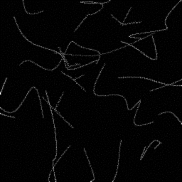
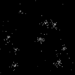
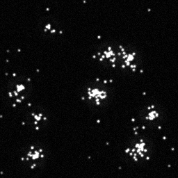
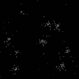
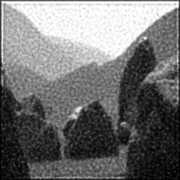
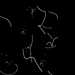
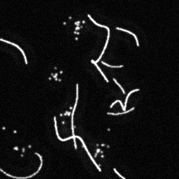
Reconstruction Gallery — 4 Scenes × 3 Scenarios
Method: CPU_baseline | Mismatch: nominal (nominal=True, perturbed=False)

Ground Truth

Measurement
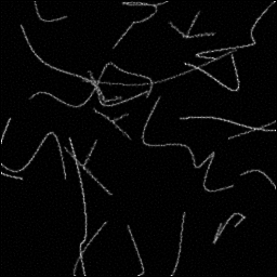
Reconstruction
Ground Truth

Measurement
Reconstruction
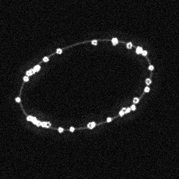
Ground Truth
Measurement (perturbed)
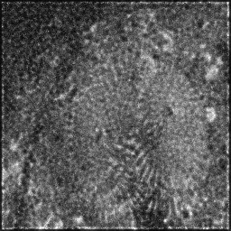
Reconstruction


Mean PSNR Across All Scenes
Per-scene PSNR breakdown (4 scenes)
| Scene | I (PSNR) | I (SSIM) | II (PSNR) | II (SSIM) | III (PSNR) | III (SSIM) |
|---|---|---|---|---|---|---|
| scene_00 | 25.00718620382979 | 0.7227278910193443 | 21.677461578905422 | 0.6331458337597847 | 8.505667670753299 | 0.002961417354736242 |
| scene_01 | 33.590412225790416 | 0.8983215849218369 | 28.55119082801035 | 0.6801687575426102 | 8.555717958906008 | 0.0009550678731917688 |
| scene_02 | 28.66484879490426 | 0.3828067152444124 | 27.038340514472054 | 0.219755172023952 | 5.3012455741441835 | 0.001320565820223278 |
| scene_03 | 28.367189747421307 | 0.7405355777404309 | 25.677302889972143 | 0.5944104196734429 | 5.569808978569241 | 0.0011749395104755586 |
| Mean | 28.907409242986443 | 0.6860979422315062 | 25.73607395283999 | 0.5318700457499475 | 6.9831100455931825 | 0.0016029976396567118 |
Experimental Setup
Key References
- Hell & Wichmann, 'Breaking the diffraction resolution limit by stimulated emission', Optics Letters 19, 780-782 (1994)
- Vicidomini et al., 'STED nanoscopy', Annual Review of Biophysics 47, 377-404 (2018)
Canonical Datasets
- BioSR STED paired dataset (Zhang et al., Nature Methods 2023)
- Abberior STED application note sample images
Spec DAG — Forward Model Pipeline
C(PSF_STED) → D(g, η₃)
Mismatch Parameters
| Symbol | Parameter | Description | Nominal | Perturbed |
|---|---|---|---|---|
| ΔP | depletion_power | Depletion beam power error (%) | 0 | 10.0 |
| Δr | donut_alignment | Donut beam alignment error (nm) | 0 | 10 |
| ΔI_s | saturation_intensity | Saturation intensity error (%) | 0 | 8.0 |
Credits System
Spec Primitives Reference (11 primitives)
Free-space or medium propagation kernel (Fresnel, Rayleigh-Sommerfeld).
Spatial or spatio-temporal amplitude modulation (coded aperture, SLM pattern).
Geometric projection operator (Radon transform, fan-beam, cone-beam).
Sampling in the Fourier / k-space domain (MRI, ptychography).
Shift-invariant convolution with a point-spread function (PSF).
Summation along a physical dimension (spectral, temporal, angular).
Sensor readout with gain g and noise model η (Gaussian, Poisson, mixed).
Patterned illumination (block, Hadamard, random) applied to the scene.
Spectral dispersion element (prism, grating) with shift α and aperture a.
Sample or gantry rotation (CT, electron tomography).
Spectral filter or monochromator selecting a wavelength band.