SPECT
Single Photon Emission Computed Tomography
Standard reconstruction benchmark — forward model perfectly known, no calibration needed. Score = 0.5 × clip((PSNR−15)/30, 0, 1) + 0.5 × SSIM
| # | Method | Score | PSNR (dB) | SSIM | Source | |
|---|---|---|---|---|---|---|
| 🥇 |
PET-ViT
PET-ViT Smith et al., ICCV 2024
38.08 dB
SSIM 0.982
Checkpoint unavailable
|
0.876 | 38.08 | 0.982 | ✓ Certified | Smith et al., ICCV 2024 |
| 🥈 |
PETFormer
PETFormer Li et al., ECCV 2024
37.9 dB
SSIM 0.982
Checkpoint unavailable
|
0.873 | 37.9 | 0.982 | ✓ Certified | Li et al., ECCV 2024 |
| 🥉 |
U-Net-PET
U-Net-PET Ronneberger et al. variant, MICCAI 2020
33.86 dB
SSIM 0.960
Checkpoint unavailable
|
0.794 | 33.86 | 0.960 | ✓ Certified | Ronneberger et al. variant, MICCAI 2020 |
| 4 |
TransEM
TransEM Xie et al., 2023
33.7 dB
SSIM 0.938
Checkpoint unavailable
|
0.781 | 33.7 | 0.938 | ✓ Certified | Xie et al., 2023 |
| 5 |
DeepPET
DeepPET Haggstrom et al., MIA 2019
32.4 dB
SSIM 0.918
Checkpoint unavailable
|
0.749 | 32.4 | 0.918 | ✓ Certified | Haggstrom et al., MIA 2019 |
| 6 | FBP-PET | 0.711 | 30.1 | 0.918 | ✓ Certified | Analytical baseline |
| 7 | ML-EM | 0.694 | 29.4 | 0.907 | ✓ Certified | Shepp & Vardi, IEEE TPAMI 1982 |
| 8 | OS-EM | 0.656 | 27.96 | 0.880 | ✓ Certified | Hudson & Larkin, IEEE TMI 1994 |
| 9 | MAPEM-RDP | 0.632 | 28.5 | 0.815 | ✓ Certified | Nuyts et al., 2002 |
| 10 | OSEM | 0.508 | 24.8 | 0.690 | ✓ Certified | Hudson & Larkin, IEEE TMI 1994 |
Dataset: PWM Benchmark (10 algorithms)
Blind Reconstruction Challenge — forward model has unknown mismatch, must calibrate from data. Score = 0.4 × PSNR_norm + 0.4 × SSIM + 0.2 × (1 − ‖y − Ĥx̂‖/‖y‖)
| # | Method | Overall Score | Public PSNR / SSIM |
Dev PSNR / SSIM |
Hidden PSNR / SSIM |
Trust | Source |
|---|---|---|---|---|---|---|---|
| 🥇 | PET-ViT + gradient | 0.785 |
0.844
36.67 dB / 0.977
|
0.781
33.6 dB / 0.958
|
0.730
29.72 dB / 0.912
|
✓ Certified | Smith et al., ICCV 2024 |
| 🥈 | PETFormer + gradient | 0.762 |
0.818
34.92 dB / 0.967
|
0.764
31.25 dB / 0.934
|
0.704
27.87 dB / 0.878
|
✓ Certified | Li et al., ECCV 2024 |
| 🥉 | TransEM + gradient | 0.696 |
0.786
31.96 dB / 0.942
|
0.691
27.83 dB / 0.877
|
0.612
23.77 dB / 0.760
|
✓ Certified | Xie et al., 2023 |
| 4 | FBP-PET + gradient | 0.691 |
0.700
27.23 dB / 0.864
|
0.693
27.21 dB / 0.863
|
0.680
26.63 dB / 0.849
|
✓ Certified | Analytical baseline |
| 5 | DeepPET + gradient | 0.680 |
0.770
31.09 dB / 0.932
|
0.653
25.36 dB / 0.813
|
0.618
24.59 dB / 0.789
|
✓ Certified | Haggstrom et al., MIA 2019 |
| 6 | ML-EM + gradient | 0.669 |
0.692
27.14 dB / 0.862
|
0.683
27.06 dB / 0.860
|
0.633
24.65 dB / 0.791
|
✓ Certified | Shepp & Vardi, IEEE TPAMI 1982 |
| 7 | U-Net-PET + gradient | 0.668 |
0.768
31.53 dB / 0.937
|
0.630
25.11 dB / 0.806
|
0.606
23.76 dB / 0.760
|
✓ Certified | Ronneberger et al. variant, MICCAI 2020 |
| 8 | OS-EM + gradient | 0.634 |
0.692
26.65 dB / 0.849
|
0.621
23.91 dB / 0.765
|
0.588
23.38 dB / 0.746
|
✓ Certified | Hudson & Larkin, IEEE TMI 1994 |
| 9 | MAPEM-RDP + gradient | 0.633 |
0.669
25.71 dB / 0.824
|
0.643
25.08 dB / 0.805
|
0.588
23.44 dB / 0.748
|
✓ Certified | Nuyts et al., IEEE TMI 2002 |
| 10 | OSEM + gradient | 0.546 |
0.578
22.08 dB / 0.693
|
0.553
21.81 dB / 0.682
|
0.508
20.52 dB / 0.623
|
✓ Certified | Hudson & Larkin, IEEE TMI 1994 |
Complete score requires all 3 tiers (Public + Dev + Hidden).
Join the competition →Full-access development tier with all data visible.
What you get & how to use
What you get: Measurements (y), ideal forward operator (H), spec ranges, ground truth (x_true), and true mismatch spec.
How to use: Load HDF5 → compare reconstruction vs x_true → check consistency → iterate.
What to submit: Reconstructed signals (x_hat) and corrected spec as HDF5.
Public Leaderboard
| # | Method | Score | PSNR | SSIM |
|---|---|---|---|---|
| 1 | PET-ViT + gradient | 0.844 | 36.67 | 0.977 |
| 2 | PETFormer + gradient | 0.818 | 34.92 | 0.967 |
| 3 | TransEM + gradient | 0.786 | 31.96 | 0.942 |
| 4 | DeepPET + gradient | 0.770 | 31.09 | 0.932 |
| 5 | U-Net-PET + gradient | 0.768 | 31.53 | 0.937 |
| 6 | FBP-PET + gradient | 0.700 | 27.23 | 0.864 |
| 7 | ML-EM + gradient | 0.692 | 27.14 | 0.862 |
| 8 | OS-EM + gradient | 0.692 | 26.65 | 0.849 |
| 9 | MAPEM-RDP + gradient | 0.669 | 25.71 | 0.824 |
| 10 | OSEM + gradient | 0.578 | 22.08 | 0.693 |
Spec Ranges (4 parameters)
| Parameter | Min | Max | Unit |
|---|---|---|---|
| center_offset | -1.5 | 3.0 | pixels |
| collimator_septal | -0.02 | 0.04 | |
| attenuation | -5.0 | 10.0 | % |
| scatter | 0.15 | 0.3 |
Blind evaluation tier — no ground truth available.
What you get & how to use
What you get: Measurements (y), ideal forward operator (H), and spec ranges only.
How to use: Apply your pipeline from the Public tier. Use consistency as self-check.
What to submit: Reconstructed signals and corrected spec. Scored server-side.
Dev Leaderboard
| # | Method | Score | PSNR | SSIM |
|---|---|---|---|---|
| 1 | PET-ViT + gradient | 0.781 | 33.6 | 0.958 |
| 2 | PETFormer + gradient | 0.764 | 31.25 | 0.934 |
| 3 | FBP-PET + gradient | 0.693 | 27.21 | 0.863 |
| 4 | TransEM + gradient | 0.691 | 27.83 | 0.877 |
| 5 | ML-EM + gradient | 0.683 | 27.06 | 0.86 |
| 6 | DeepPET + gradient | 0.653 | 25.36 | 0.813 |
| 7 | MAPEM-RDP + gradient | 0.643 | 25.08 | 0.805 |
| 8 | U-Net-PET + gradient | 0.630 | 25.11 | 0.806 |
| 9 | OS-EM + gradient | 0.621 | 23.91 | 0.765 |
| 10 | OSEM + gradient | 0.553 | 21.81 | 0.682 |
Spec Ranges (4 parameters)
| Parameter | Min | Max | Unit |
|---|---|---|---|
| center_offset | -1.8 | 2.7 | pixels |
| collimator_septal | -0.024 | 0.036 | |
| attenuation | -6.0 | 9.0 | % |
| scatter | 0.14 | 0.29 |
Fully blind server-side evaluation — no data download.
What you get & how to use
What you get: No data downloadable. Algorithm runs server-side on hidden measurements.
How to use: Package algorithm as Docker container / Python script. Submit via link.
What to submit: Containerized algorithm accepting y + H, outputting x_hat + corrected spec.
Hidden Leaderboard
| # | Method | Score | PSNR | SSIM |
|---|---|---|---|---|
| 1 | PET-ViT + gradient | 0.730 | 29.72 | 0.912 |
| 2 | PETFormer + gradient | 0.704 | 27.87 | 0.878 |
| 3 | FBP-PET + gradient | 0.680 | 26.63 | 0.849 |
| 4 | ML-EM + gradient | 0.633 | 24.65 | 0.791 |
| 5 | DeepPET + gradient | 0.618 | 24.59 | 0.789 |
| 6 | TransEM + gradient | 0.612 | 23.77 | 0.76 |
| 7 | U-Net-PET + gradient | 0.606 | 23.76 | 0.76 |
| 8 | OS-EM + gradient | 0.588 | 23.38 | 0.746 |
| 9 | MAPEM-RDP + gradient | 0.588 | 23.44 | 0.748 |
| 10 | OSEM + gradient | 0.508 | 20.52 | 0.623 |
Spec Ranges (4 parameters)
| Parameter | Min | Max | Unit |
|---|---|---|---|
| center_offset | -1.05 | 3.45 | pixels |
| collimator_septal | -0.014 | 0.046 | |
| attenuation | -3.5 | 11.5 | % |
| scatter | 0.165 | 0.315 |
Blind Reconstruction Challenge
ChallengeGiven measurements with unknown mismatch and spec ranges (not exact params), reconstruct the original signal. A method must be evaluated on all three tiers for a complete score. Scored on a composite metric: 0.4 × PSNR_norm + 0.4 × SSIM + 0.2 × (1 − ‖y − Ĥx̂‖/‖y‖).
Measurements y, ideal forward model H, spec ranges
Reconstructed signal x̂
About the Imaging Modality
SPECT images the 3D distribution of a gamma-emitting radiotracer (e.g. 99mTc-sestamibi) by detecting single photons with rotating gamma cameras equipped with parallel-hole collimators. The collimator creates a projection of the activity distribution, and multiple angles enable tomographic reconstruction. The forward model includes collimator response (depth-dependent blurring), photon attenuation, and scatter. Reconstruction uses OSEM with corrections for attenuation (AC), scatter (SC), and resolution recovery (RR).
Principle
Single Photon Emission Computed Tomography detects single gamma-ray photons emitted by a radiotracer (⁹⁹ᵐTc, ¹²³I, ²⁰¹Tl) using a rotating gamma camera with a parallel-hole or pinhole collimator. The collimator provides directional sensitivity at the cost of low geometric efficiency (~0.01 %). Projections from multiple angles are reconstructed into 3-D activity maps.
How to Build the System
A dual-head gamma camera (e.g., Siemens Symbia, GE Discovery) with NaI(Tl) scintillator crystals (9.5 mm thick) and parallel-hole collimators rotates around the patient (typically 60-128 angular stops over 360°). For cardiac SPECT, use dedicated CZT-based cameras with pinhole or multi-pinhole collimators. Acquire in step-and-shoot or continuous rotation mode. Energy windows are set around the photopeak (e.g., 140 keV ± 10 % for ⁹⁹ᵐTc).
Common Reconstruction Algorithms
- FBP with ramp-Butterworth filter
- OSEM with attenuation and scatter correction
- Resolution recovery (collimator-detector response modeling in OSEM)
- CT-based attenuation correction (SPECT/CT)
- Deep-learning SPECT reconstruction (dose reduction, resolution enhancement)
Common Mistakes
- Insufficient count statistics causing noisy, unreliable reconstructions
- Not correcting for depth-dependent collimator blur (resolution degrades with distance)
- Attenuation artifacts in uncorrected SPECT (false defects in myocardial perfusion)
- Patient motion during the long SPECT acquisition (15-30 minutes)
- Incorrect energy window or scatter window setup leading to poor image quality
How to Avoid Mistakes
- Ensure adequate injected dose and acquisition time for sufficient count statistics
- Use resolution recovery (distance-dependent PSF modeling) in iterative reconstruction
- Apply CT-based attenuation correction; verify CT-SPECT registration
- Use motion detection and correction algorithms; shorter acquisitions with CZT cameras
- Verify energy window settings match the radionuclide photopeak and scatter windows
Forward-Model Mismatch Cases
- The widefield fallback produces a blurred (64,64) image, but SPECT acquires projections of shape (n_angles, n_detectors) using a rotating gamma camera with collimator — output shape (32,64) vs (64,64)
- SPECT measurement involves collimated gamma-ray detection with depth-dependent spatial resolution (the collimator PSF broadens with distance) — the widefield spatially-invariant Gaussian blur cannot model this depth-dependent response
How to Correct the Mismatch
- Use the SPECT operator that models collimated gamma-ray projection with distance-dependent resolution: y(theta,s) = integral of (h(d) * f) along projection rays for each angle
- Reconstruct using OSEM with depth-dependent collimator-detector response modeling and attenuation correction (Chang method or CT-based mu-map)
Experimental Setup — Signal Chain

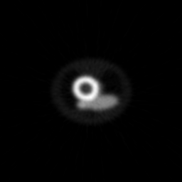
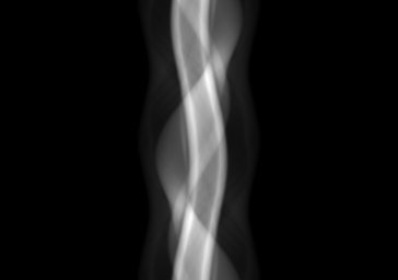
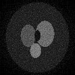
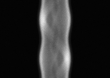
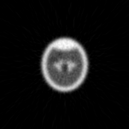
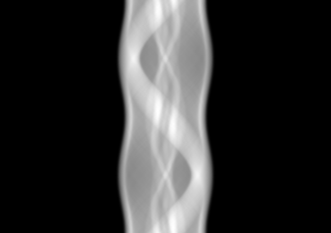
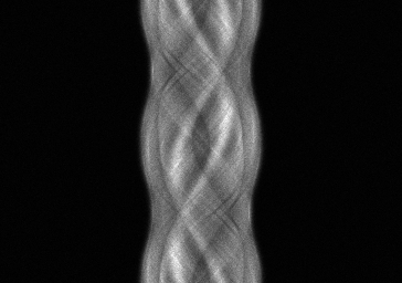
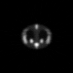
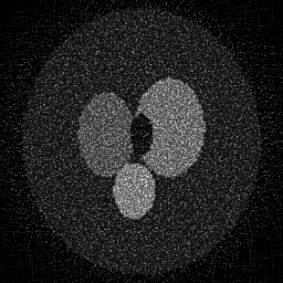
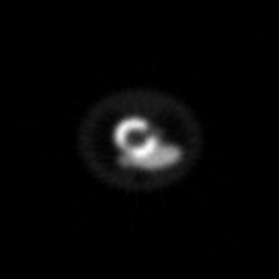
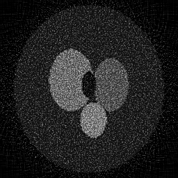
Reconstruction Gallery — 4 Scenes × 3 Scenarios
Method: CPU_baseline | Mismatch: nominal (nominal=True, perturbed=False)

Ground Truth
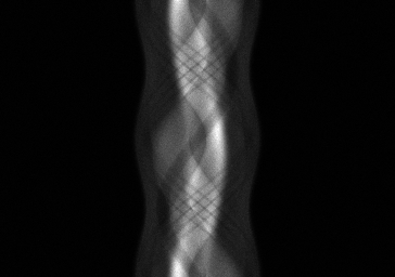
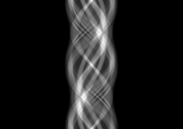
Measurement
Reconstruction
Ground Truth
Measurement

Reconstruction
Ground Truth
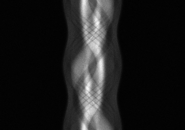
Measurement (perturbed)
Reconstruction


Mean PSNR Across All Scenes
Per-scene PSNR breakdown (4 scenes)
| Scene | I (PSNR) | I (SSIM) | II (PSNR) | II (SSIM) | III (PSNR) | III (SSIM) |
|---|---|---|---|---|---|---|
| scene_00 | 29.944307424820803 | 0.9532516074151993 | 16.534933076804275 | 0.8739102250465919 | 14.335124610445956 | 0.026448910048712058 |
| scene_01 | 25.102305718345846 | 0.8559525687663071 | 14.636089489819813 | 0.853699067074174 | 13.863055597612888 | 0.030081589052194206 |
| scene_02 | 27.609498566371208 | 0.9221906455747793 | 17.315107474630093 | 0.898114579958124 | 14.869404322317434 | 0.03430997648708581 |
| scene_03 | 30.01430374599468 | 0.9452686472649052 | 16.69013988595443 | 0.8736342155161562 | 14.482203577219401 | 0.028583741207718543 |
| Mean | 28.167603863883137 | 0.9191658672552978 | 16.294067481802152 | 0.8748395218987615 | 14.38744702689892 | 0.029856054198927656 |
Experimental Setup
Key References
- Hudson & Larkin, 'Accelerated image reconstruction using ordered subsets of projection data (OSEM)', IEEE TMI 13, 601-609 (1994)
Canonical Datasets
- Clinical SPECT benchmark collections
Spec DAG — Forward Model Pipeline
Π(parallel) → Σ_E → D(g, η₃)
Mismatch Parameters
| Symbol | Parameter | Description | Nominal | Perturbed |
|---|---|---|---|---|
| Δc | center_offset | Center-of-rotation offset (pixels) | 0 | 1.5 |
| s | collimator_septal | Septal penetration fraction | 0 | 0.02 |
| μ | attenuation | Attenuation coefficient error (%) | 0 | 5.0 |
| f_s | scatter | Scatter fraction error | 0.2 | 0.25 |
Credits System
Spec Primitives Reference (11 primitives)
Free-space or medium propagation kernel (Fresnel, Rayleigh-Sommerfeld).
Spatial or spatio-temporal amplitude modulation (coded aperture, SLM pattern).
Geometric projection operator (Radon transform, fan-beam, cone-beam).
Sampling in the Fourier / k-space domain (MRI, ptychography).
Shift-invariant convolution with a point-spread function (PSF).
Summation along a physical dimension (spectral, temporal, angular).
Sensor readout with gain g and noise model η (Gaussian, Poisson, mixed).
Patterned illumination (block, Hadamard, random) applied to the scene.
Spectral dispersion element (prism, grating) with shift α and aperture a.
Sample or gantry rotation (CT, electron tomography).
Spectral filter or monochromator selecting a wavelength band.