SPC-Block
Single-Pixel Camera (Block Sensing)
Standard reconstruction benchmark — forward model perfectly known, no calibration needed. Score = 0.5 × clip((PSNR−15)/30, 0, 1) + 0.5 × SSIM
| # | Method | Score | PSNR (dB) | SSIM | Source | |
|---|---|---|---|---|---|---|
| 🥇 | HATNet | 0.731 | 28.85 | 0.801 | ✓ Certified | InverseNet baseline (oracle cal) |
| 🥈 | ISTA-Net+ | 0.710 | 27.56 | 0.762 | ✓ Certified | ISTA-Net+ (CVPR 2018) |
| 🥉 | FISTA-TV | 0.686 | 26.1 | 0.758 | ✓ Certified | InverseNet baseline (oracle cal) |
| 4 | PnP-DRUNet | 0.632 | 23.85 | 0.665 | ✓ Certified | InverseNet baseline (oracle cal) |
Dataset: Set11, block 33×33, CR=0.25
Blind Reconstruction Challenge — forward model has unknown mismatch, must calibrate from data. Score = 0.4 × PSNR_norm + 0.4 × SSIM + 0.2 × (1 − ‖y − Ĥx̂‖/‖y‖)
| # | Method | Overall Score | Public PSNR / SSIM |
Dev PSNR / SSIM |
Hidden PSNR / SSIM |
Trust | Source |
|---|---|---|---|---|---|---|---|
| 🥇 | HATNet + gradient | 0.651 |
0.710
27.91 dB / 0.778
|
0.630
23.34 dB / 0.708
|
0.612
22.51 dB / 0.696
|
✓ Certified | InverseNet baseline |
| 🥈 | ISTA-Net + gradient | 0.647 |
0.694
26.61 dB / 0.742
|
0.634
23.66 dB / 0.681
|
0.614
22.81 dB / 0.663
|
✓ Certified | InverseNet baseline |
| 🥉 | FISTA-TV + gradient | 0.633 |
0.680
25.29 dB / 0.738
|
0.618
22.51 dB / 0.676
|
0.600
21.74 dB / 0.659
|
✓ Certified | InverseNet baseline |
| 4 | PnP-DRUNet + gradient | 0.575 |
0.627
22.99 dB / 0.643
|
0.560
20.41 dB / 0.556
|
0.537
19.68 dB / 0.530
|
✓ Certified | InverseNet baseline |
Complete score requires all 3 tiers (Public + Dev + Hidden).
Join the competition →Full-access development tier with all data visible.
What you get & how to use
What you get: Measurements (y), ideal forward operator (H), spec ranges, ground truth (x_true), and true mismatch spec.
How to use: Load HDF5 → compare reconstruction vs x_true → check consistency → iterate.
What to submit: Reconstructed signals (x_hat) and corrected spec as HDF5.
Public Leaderboard
| # | Method | Score | PSNR | SSIM |
|---|---|---|---|---|
| 1 | HATNet + gradient | 0.710 | 27.91 | 0.778 |
| 2 | ISTA-Net + gradient | 0.694 | 26.61 | 0.742 |
| 3 | FISTA-TV + gradient | 0.680 | 25.29 | 0.738 |
| 4 | PnP-DRUNet + gradient | 0.627 | 22.99 | 0.643 |
Spec Ranges (2 parameters)
| Parameter | Min | Max | Unit |
|---|---|---|---|
| gain_decay_alpha | 0.0005 | 0.0095 | 1/measurement |
| noise_sigma | 0.01 | 0.05 |
Blind evaluation tier — no ground truth available.
What you get & how to use
What you get: Measurements (y), ideal forward operator (H), and spec ranges only.
How to use: Apply your pipeline from the Public tier. Use consistency as self-check.
What to submit: Reconstructed signals and corrected spec. Scored server-side.
Dev Leaderboard
| # | Method | Score | PSNR | SSIM |
|---|---|---|---|---|
| 1 | ISTA-Net + gradient | 0.634 | 23.66 | 0.681 |
| 2 | HATNet + gradient | 0.630 | 23.34 | 0.708 |
| 3 | FISTA-TV + gradient | 0.618 | 22.51 | 0.676 |
| 4 | PnP-DRUNet + gradient | 0.560 | 20.41 | 0.556 |
Spec Ranges (2 parameters)
| Parameter | Min | Max | Unit |
|---|---|---|---|
| gain_decay_alpha | -0.0015 | 0.0075 | 1/measurement |
| noise_sigma | 0.0 | 0.04 |
Fully blind server-side evaluation — no data download.
What you get & how to use
What you get: No data downloadable. Algorithm runs server-side on hidden measurements.
How to use: Package algorithm as Docker container / Python script. Submit via link.
What to submit: Containerized algorithm accepting y + H, outputting x_hat + corrected spec.
Hidden Leaderboard
| # | Method | Score | PSNR | SSIM |
|---|---|---|---|---|
| 1 | ISTA-Net + gradient | 0.614 | 22.81 | 0.663 |
| 2 | HATNet + gradient | 0.612 | 22.51 | 0.696 |
| 3 | FISTA-TV + gradient | 0.600 | 21.74 | 0.659 |
| 4 | PnP-DRUNet + gradient | 0.537 | 19.68 | 0.53 |
Spec Ranges (2 parameters)
| Parameter | Min | Max | Unit |
|---|---|---|---|
| gain_decay_alpha | 0.0035 | 0.0125 | 1/measurement |
| noise_sigma | 0.02 | 0.06 |
Blind Reconstruction Challenge
ChallengeGiven measurements with unknown mismatch and spec ranges (not exact params), reconstruct the original signal. A method must be evaluated on all three tiers for a complete score. Scored on a composite metric: 0.4 × PSNR_norm + 0.4 × SSIM + 0.2 × (1 − ‖y − Ĥx̂‖/‖y‖).
Measurements y, ideal forward model H, spec ranges
Reconstructed signal x̂
About the Imaging Modality
The single-pixel camera reconstructs a 2D image from scalar intensity measurements acquired by a photodiode after spatially modulating the scene with known patterns on a DMD. Each measurement y_i is the inner product of the scene with a pattern, giving y = Phi*x + n. Compressed sensing theory guarantees recovery from M << N measurements if the scene is sparse. The single detector can operate at wavelengths where array detectors are unavailable (SWIR, THz). Reconstruction uses FISTA with L1/TV penalties or Plug-and-Play methods.
Principle
A single-pixel camera uses a spatial light modulator (DMD) to project a sequence of binary or grayscale patterns onto the scene. Each pattern multiplies the scene, and a single bucket detector (photodiode or PMT) measures the total light for each pattern, producing one scalar measurement per pattern. Compressive sensing recovers the image from far fewer measurements than Nyquist by exploiting sparsity in a transform domain.
How to Build the System
Place a DMD (e.g., Texas Instruments DLP LightCrafter) at the image plane of a relay lens. Focus the scene onto the DMD. After the DMD, collect all reflected light onto a single photodetector (avalanche photodiode for low light, or silicon photodiode for visible). Display Hadamard, random, or optimized patterns at 10-22 kHz DMD rate. Synchronize pattern display with detector readout.
Common Reconstruction Algorithms
- Basis pursuit / L1 minimization (LASSO)
- Orthogonal matching pursuit (OMP)
- Total-variation minimization (TV-CS)
- TVAL3 (TV with augmented Lagrangian and alternating direction)
- Deep compressive sensing networks (ReconNet, CSNet)
Common Mistakes
- Pattern-detector timing mismatch causing wrong measurement-to-pattern association
- DMD diffraction effects not accounted for at oblique illumination angles
- Insufficient measurements for the scene complexity (under-sampling ratio too aggressive)
- Analog-to-digital converter resolution too low for the dynamic range of measurements
- Not calibrating detector linearity and dark current drift during long acquisitions
How to Avoid Mistakes
- Hardware-trigger the detector acquisition from the DMD synchronization signal
- Calibrate the effective pattern at the sample plane (not just the DMD command pattern)
- Start with 25-50 % measurement ratio for natural scenes; reduce only if sparsity allows
- Use 16-bit or higher ADC; verify linearity with a calibrated light source
- Measure dark frames periodically and subtract; maintain stable detector temperature
Forward-Model Mismatch Cases
- The widefield fallback produces a 2D (64,64) image, but single-pixel camera acquires a 1D vector of M scalar measurements (M << N pixels) via structured illumination patterns and a single photodetector — output shape (M,) vs (64,64)
- Each SPC measurement is an inner product of the scene with a known pattern (y_i = <phi_i, x>), capturing compressed information — the widefield blur produces N^2 pixels with no compression, making compressive reconstruction algorithms incompatible
How to Correct the Mismatch
- Use the SPC operator that applies the sensing matrix Phi (Hadamard, random, or learned patterns): y = Phi * x, where y has far fewer entries than the image has pixels
- Reconstruct using compressive sensing algorithms (ISTA-Net, basis pursuit, total variation) that exploit sparsity to recover the N^2-pixel image from M << N^2 measurements
Experimental Setup — Signal Chain

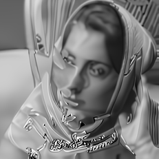
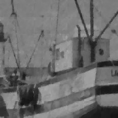
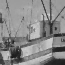
Reconstruction Gallery — 4 Scenes × 3 Scenarios
Method: CPU_baseline | Mismatch: nominal (nominal=True, perturbed=False)

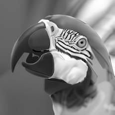
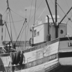
Ground Truth
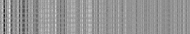
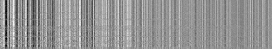
Measurement
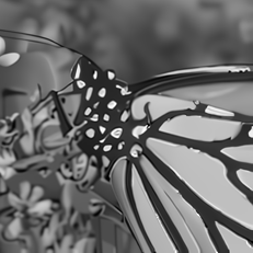
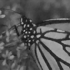
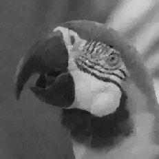
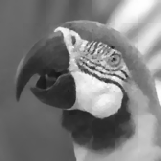
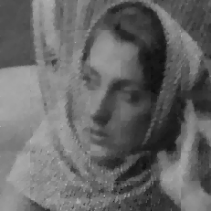
Reconstruction
Ground Truth

Measurement
Reconstruction
Ground Truth
Measurement (perturbed)

Reconstruction


Mean PSNR Across All Scenes
Per-scene PSNR breakdown (4 scenes)
| Scene | I (PSNR) | I (SSIM) | II (PSNR) | II (SSIM) | III (PSNR) | III (SSIM) |
|---|---|---|---|---|---|---|
| scene_00 | 25.39371707885856 | 0.8480747085041821 | 18.820022565491644 | 0.7840283295335593 | 26.511274217147033 | 0.8618602929670134 |
| scene_01 | 27.01470648489959 | 0.8492677765876193 | 18.37263138756575 | 0.7962725053613845 | 26.515625207621092 | 0.8633560142161486 |
| scene_02 | 21.78365670394792 | 0.6938984144887997 | 17.98799113843805 | 0.6610216572963897 | 24.858503006256733 | 0.7310837438769546 |
| scene_03 | 26.509906102931765 | 0.8000791806834071 | 18.064524965376286 | 0.7181165510121686 | 27.396775993761086 | 0.797057961697343 |
| Mean | 25.17549659265946 | 0.797830020066002 | 18.311292514217932 | 0.7398597608008755 | 26.320544606196485 | 0.8133395031893649 |
Experimental Setup
Key References
- Duarte et al., 'Single-pixel imaging via compressive sampling', IEEE Signal Processing Magazine 25, 83-91 (2008)
- Edgar et al., 'Principles and prospects for single-pixel imaging', Nature Photonics 13, 13-20 (2019)
Canonical Datasets
- Set11 (11 standard test images)
- BSD68 (Martin et al., ICCV 2001)
Spec DAG — Forward Model Pipeline
S(block) → M(Φ) → Σ → D(g, η₁)
Mismatch Parameters
| Symbol | Parameter | Description | Nominal | Perturbed |
|---|---|---|---|---|
| α | gain_alpha | Gain drift coefficient | 0 | 0.0015 |
| σ_y | sigma_y | Measurement noise std | 0 | 0.03 |
Credits System
Spec Primitives Reference (11 primitives)
Free-space or medium propagation kernel (Fresnel, Rayleigh-Sommerfeld).
Spatial or spatio-temporal amplitude modulation (coded aperture, SLM pattern).
Geometric projection operator (Radon transform, fan-beam, cone-beam).
Sampling in the Fourier / k-space domain (MRI, ptychography).
Shift-invariant convolution with a point-spread function (PSF).
Summation along a physical dimension (spectral, temporal, angular).
Sensor readout with gain g and noise model η (Gaussian, Poisson, mixed).
Patterned illumination (block, Hadamard, random) applied to the scene.
Spectral dispersion element (prism, grating) with shift α and aperture a.
Sample or gantry rotation (CT, electron tomography).
Spectral filter or monochromator selecting a wavelength band.