SIM
Structured Illumination Microscopy
Standard reconstruction benchmark — forward model perfectly known, no calibration needed. Score = 0.5 × clip((PSNR−15)/30, 0, 1) + 0.5 × SSIM
| # | Method | Score | PSNR (dB) | SSIM | Source | |
|---|---|---|---|---|---|---|
| 🥇 |
SIMformer
SIMformer SIM reconstruction transformer, 2024
36.5 dB
SSIM 0.960
Checkpoint unavailable
|
0.838 | 36.5 | 0.960 | ✓ Certified | SIM reconstruction transformer, 2024 |
| 🥈 |
DL-SIM
DL-SIM Jin et al., Nat. Methods 2023
35.0 dB
SSIM 0.945
Checkpoint unavailable
|
0.806 | 35.0 | 0.945 | ✓ Certified | Jin et al., Nat. Methods 2023 |
| 🥉 | PnP-SIM | 0.720 | 31.5 | 0.890 | ✓ Certified | PnP with SIM forward model |
| 4 | Wiener-SIM | 0.635 | 28.5 | 0.820 | ✓ Certified | Gustafsson, J. Microsc. 2000 |
Dataset: PWM Benchmark (4 algorithms)
Blind Reconstruction Challenge — forward model has unknown mismatch, must calibrate from data. Score = 0.4 × PSNR_norm + 0.4 × SSIM + 0.2 × (1 − ‖y − Ĥx̂‖/‖y‖)
| # | Method | Overall Score | Public PSNR / SSIM |
Dev PSNR / SSIM |
Hidden PSNR / SSIM |
Trust | Source |
|---|---|---|---|---|---|---|---|
| 🥇 | SIMformer + gradient | 0.773 |
0.805
34.37 dB / 0.964
|
0.791
33.78 dB / 0.959
|
0.723
29.38 dB / 0.907
|
✓ Certified | SIM reconstruction transformer, 2024 |
| 🥈 | DL-SIM + gradient | 0.676 |
0.785
33.01 dB / 0.953
|
0.660
25.49 dB / 0.817
|
0.584
22.81 dB / 0.724
|
✓ Certified | Jin et al., Nat. Methods 2023 |
| 🥉 | PnP-SIM + gradient | 0.660 |
0.731
29.3 dB / 0.906
|
0.648
25.21 dB / 0.809
|
0.600
24.01 dB / 0.769
|
✓ Certified | PnP with SIM forward model |
| 4 | Wiener-SIM + gradient | 0.658 |
0.698
26.85 dB / 0.854
|
0.662
26.24 dB / 0.839
|
0.615
23.97 dB / 0.767
|
✓ Certified | Gustafsson, J. Microsc. 2000 |
Complete score requires all 3 tiers (Public + Dev + Hidden).
Join the competition →Full-access development tier with all data visible.
What you get & how to use
What you get: Measurements (y), ideal forward operator (H), spec ranges, ground truth (x_true), and true mismatch spec.
How to use: Load HDF5 → compare reconstruction vs x_true → check consistency → iterate.
What to submit: Reconstructed signals (x_hat) and corrected spec as HDF5.
Public Leaderboard
| # | Method | Score | PSNR | SSIM |
|---|---|---|---|---|
| 1 | SIMformer + gradient | 0.805 | 34.37 | 0.964 |
| 2 | DL-SIM + gradient | 0.785 | 33.01 | 0.953 |
| 3 | PnP-SIM + gradient | 0.731 | 29.3 | 0.906 |
| 4 | Wiener-SIM + gradient | 0.698 | 26.85 | 0.854 |
Spec Ranges (3 parameters)
| Parameter | Min | Max | Unit |
|---|---|---|---|
| pattern_phase | -0.05 | 0.1 | rad |
| pattern_freq | -1.0 | 2.0 | % |
| modulation_depth | -5.0 | 10.0 | % |
Blind evaluation tier — no ground truth available.
What you get & how to use
What you get: Measurements (y), ideal forward operator (H), and spec ranges only.
How to use: Apply your pipeline from the Public tier. Use consistency as self-check.
What to submit: Reconstructed signals and corrected spec. Scored server-side.
Dev Leaderboard
| # | Method | Score | PSNR | SSIM |
|---|---|---|---|---|
| 1 | SIMformer + gradient | 0.791 | 33.78 | 0.959 |
| 2 | Wiener-SIM + gradient | 0.662 | 26.24 | 0.839 |
| 3 | DL-SIM + gradient | 0.660 | 25.49 | 0.817 |
| 4 | PnP-SIM + gradient | 0.648 | 25.21 | 0.809 |
Spec Ranges (3 parameters)
| Parameter | Min | Max | Unit |
|---|---|---|---|
| pattern_phase | -0.06 | 0.09 | rad |
| pattern_freq | -1.2 | 1.8 | % |
| modulation_depth | -6.0 | 9.0 | % |
Fully blind server-side evaluation — no data download.
What you get & how to use
What you get: No data downloadable. Algorithm runs server-side on hidden measurements.
How to use: Package algorithm as Docker container / Python script. Submit via link.
What to submit: Containerized algorithm accepting y + H, outputting x_hat + corrected spec.
Hidden Leaderboard
| # | Method | Score | PSNR | SSIM |
|---|---|---|---|---|
| 1 | SIMformer + gradient | 0.723 | 29.38 | 0.907 |
| 2 | Wiener-SIM + gradient | 0.615 | 23.97 | 0.767 |
| 3 | PnP-SIM + gradient | 0.600 | 24.01 | 0.769 |
| 4 | DL-SIM + gradient | 0.584 | 22.81 | 0.724 |
Spec Ranges (3 parameters)
| Parameter | Min | Max | Unit |
|---|---|---|---|
| pattern_phase | -0.035 | 0.115 | rad |
| pattern_freq | -0.7 | 2.3 | % |
| modulation_depth | -3.5 | 11.5 | % |
Blind Reconstruction Challenge
ChallengeGiven measurements with unknown mismatch and spec ranges (not exact params), reconstruct the original signal. A method must be evaluated on all three tiers for a complete score. Scored on a composite metric: 0.4 × PSNR_norm + 0.4 × SSIM + 0.2 × (1 − ‖y − Ĥx̂‖/‖y‖).
Measurements y, ideal forward model H, spec ranges
Reconstructed signal x̂
About the Imaging Modality
Structured illumination microscopy (SIM) achieves ~2x lateral resolution improvement by illuminating the sample with sinusoidal patterns at multiple orientations and phases. Frequency mixing between the illumination pattern and sample structure shifts high-frequency information into the microscope passband. Reconstruction separates and reassembles frequency components via Wiener-SIM or deep-learning SIM. The forward model is y_k = PSF ** (I_k * x) + n for each pattern k.
Principle
Structured Illumination Microscopy projects a known sinusoidal pattern onto the specimen, shifting high-frequency spatial information into the observable passband via Moiré interference. Multiple images (typically 9-15) are acquired at different pattern orientations and phases, then computationally recombined in Fourier space to achieve ~2× lateral resolution improvement beyond the diffraction limit.
How to Build the System
Install a SIM-capable microscope (Nikon N-SIM, Zeiss Elyra 7, or custom with SLM/DMD). Use a high-NA objective (100x 1.49 NA TIRF) for maximum frequency extension. The illumination grating (SLM or fiber interference) generates the sinusoidal pattern. Acquire 3 orientations × 3-5 phases. A fast sCMOS camera captures all raw frames in ~100-500 ms for 2D-SIM. Careful alignment of the pattern contrast is critical.
Common Reconstruction Algorithms
- Gustafsson/Heintzmann frequency-domain SIM reconstruction
- Open-source fairSIM (ImageJ plugin)
- Wiener-filtered order separation and recombination
- Deep-learning SIM (ML-SIM, reconstruction from fewer frames)
- Hessian-SIM for live-cell with reduced artifacts
Common Mistakes
- Insufficient pattern contrast causing weak Moiré fringes and honeycomb artifacts
- Misaligned illumination orders producing stripe artifacts in the reconstruction
- Over-processing (too aggressive Wiener parameter) creating ringing artifacts
- Using objectives with insufficient NA for the desired resolution gain
- Photobleaching between pattern acquisitions causing intensity inconsistency
How to Avoid Mistakes
- Verify pattern contrast >0.5 on a thin uniform fluorescent layer before experiments
- Calibrate illumination pattern positions/angles using SIMcheck (ImageJ plugin)
- Tune the Wiener parameter conservatively; use SIMcheck to assess reconstruction quality
- Use 1.49 NA objectives for maximum resolution; 1.40 NA limits SIM performance
- Minimize total acquisition time; use fast cameras and short exposures
Forward-Model Mismatch Cases
- The widefield fallback produces a single (64,64) blurred image, but SIM requires 9-15 raw frames (3 orientations x 3-5 phases) with structured illumination patterns — output shape (64,64,9) vs (64,64)
- Without the sinusoidal illumination pattern encoding, the high-frequency information that SIM moves into the passband via Moiré interference is completely absent — no super-resolution is possible
How to Correct the Mismatch
- Use the SIM operator that generates multiple pattern-modulated images: y_k = (1 + m*cos(k_i*r + phi_j)) * (PSF ** x) for each orientation i and phase j
- Reconstruct using Fourier-space order separation and recombination (Gustafsson method) or deep-learning SIM, which require the correct multi-frame structured illumination forward model
Experimental Setup — Signal Chain

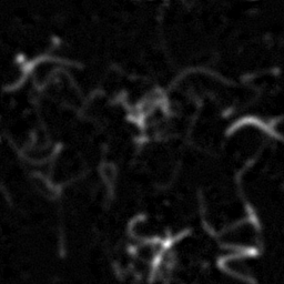
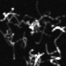
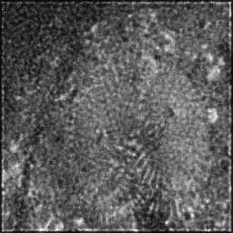
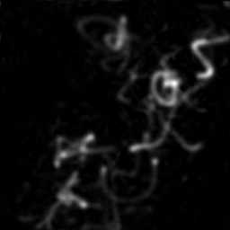
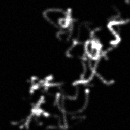
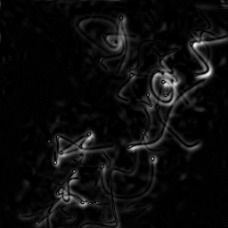
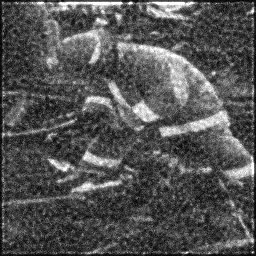
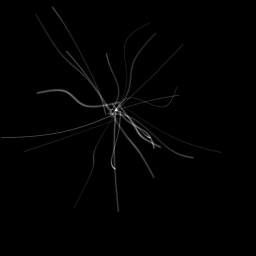
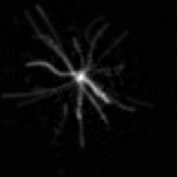
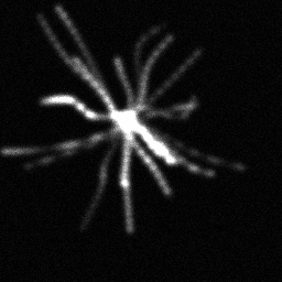
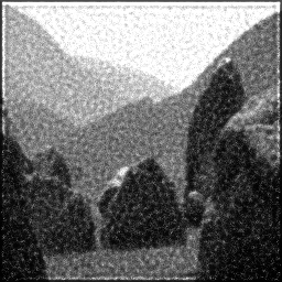
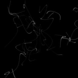
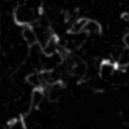
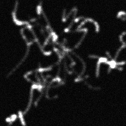
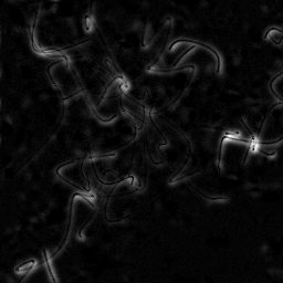
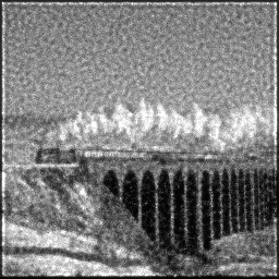
Reconstruction Gallery — 4 Scenes × 3 Scenarios
Method: CPU_baseline | Mismatch: nominal (nominal=True, perturbed=False)
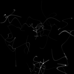
Ground Truth

Measurement
Reconstruction
Ground Truth
Measurement

Reconstruction
Ground Truth
Measurement (perturbed)
Reconstruction


Mean PSNR Across All Scenes
Per-scene PSNR breakdown (4 scenes)
| Scene | I (PSNR) | I (SSIM) | II (PSNR) | II (SSIM) | III (PSNR) | III (SSIM) |
|---|---|---|---|---|---|---|
| scene_00 | 21.658016625070744 | 0.18898242665750162 | 21.170493444304856 | 0.08187590065722772 | 8.449277632080424 | 0.00435169404607965 |
| scene_01 | 23.6369128699697 | 0.5874743745514779 | 20.697100936560968 | 0.31416577539287693 | 8.7727063459029 | 0.004366784033425171 |
| scene_02 | 24.77095580046018 | 0.5135595254425513 | 24.52118543687586 | 0.42127165975522035 | 5.363591347780973 | 0.0029944343687771887 |
| scene_03 | 22.250938413151104 | 0.25747941084571485 | 21.618998887742094 | 0.1494503500511923 | 5.598019973001863 | 0.002744020990484861 |
| Mean | 23.07920592716293 | 0.3868739343743114 | 22.001944676370947 | 0.24169092146412935 | 7.045898824691539 | 0.0036142333596917175 |
Experimental Setup
Key References
- Gustafsson, 'Surpassing the lateral resolution limit by a factor of two using structured illumination microscopy', J. Microsc. 198, 82-87 (2000)
- Muller & Bhatt, 'Open-source image reconstruction of super-resolution structured illumination microscopy data (fairSIM)', Nature Comms 7, 10980 (2016)
Canonical Datasets
- BioSR SIM paired dataset (Zhang et al., Nature Methods 2023)
- fairSIM test datasets (Hagen et al.)
Spec DAG — Forward Model Pipeline
S(grating) → C(PSF) → Σ_φ → D(g, η₃)
Mismatch Parameters
| Symbol | Parameter | Description | Nominal | Perturbed |
|---|---|---|---|---|
| Δφ | pattern_phase | Pattern phase error (rad) | 0 | 0.05 |
| Δk | pattern_freq | Pattern frequency error (%) | 0 | 1.0 |
| Δm | modulation_depth | Modulation depth error (%) | 0 | 5.0 |
Credits System
Spec Primitives Reference (11 primitives)
Free-space or medium propagation kernel (Fresnel, Rayleigh-Sommerfeld).
Spatial or spatio-temporal amplitude modulation (coded aperture, SLM pattern).
Geometric projection operator (Radon transform, fan-beam, cone-beam).
Sampling in the Fourier / k-space domain (MRI, ptychography).
Shift-invariant convolution with a point-spread function (PSF).
Summation along a physical dimension (spectral, temporal, angular).
Sensor readout with gain g and noise model η (Gaussian, Poisson, mixed).
Patterned illumination (block, Hadamard, random) applied to the scene.
Spectral dispersion element (prism, grating) with shift α and aperture a.
Sample or gantry rotation (CT, electron tomography).
Spectral filter or monochromator selecting a wavelength band.