SEM
Scanning Electron Microscopy
Standard reconstruction benchmark — forward model perfectly known, no calibration needed. Score = 0.5 × clip((PSNR−15)/30, 0, 1) + 0.5 × SSIM
| # | Method | Score | PSNR (dB) | SSIM | Source | |
|---|---|---|---|---|---|---|
| 🥇 |
SwinIR
SwinIR Liang et al., ICCVW 2021
33.4 dB
SSIM 0.930
Checkpoint unavailable
|
0.772 | 33.4 | 0.930 | ✓ Certified | Liang et al., ICCVW 2021 |
| 🥈 |
Noise2Void
Noise2Void Krull et al., CVPR 2019
31.6 dB
SSIM 0.895
Checkpoint unavailable
|
0.724 | 31.6 | 0.895 | ✓ Certified | Krull et al., CVPR 2019 |
| 🥉 | BM3D | 0.635 | 28.5 | 0.820 | ✓ Certified | Dabov et al., IEEE TIP 2007 |
| 4 | Wiener Filter | 0.503 | 24.8 | 0.680 | ✓ Certified | Analytical baseline |
Dataset: PWM Benchmark (4 algorithms)
Blind Reconstruction Challenge — forward model has unknown mismatch, must calibrate from data. Score = 0.4 × PSNR_norm + 0.4 × SSIM + 0.2 × (1 − ‖y − Ĥx̂‖/‖y‖)
| # | Method | Overall Score | Public PSNR / SSIM |
Dev PSNR / SSIM |
Hidden PSNR / SSIM |
Trust | Source |
|---|---|---|---|---|---|---|---|
| 🥇 | SwinIR + gradient | 0.713 |
0.763
31.55 dB / 0.938
|
0.716
29.08 dB / 0.902
|
0.661
26.38 dB / 0.842
|
✓ Certified | Liang et al., ICCVW 2021 |
| 🥈 | Noise2Void + gradient | 0.567 |
0.735
29.74 dB / 0.913
|
0.525
20.46 dB / 0.621
|
0.441
17.75 dB / 0.488
|
✓ Certified | Krull et al., CVPR 2019 |
| 🥉 | BM3D + gradient | 0.565 |
0.669
25.73 dB / 0.824
|
0.564
22.23 dB / 0.700
|
0.463
18.42 dB / 0.521
|
✓ Certified | Dabov et al., IEEE TIP 2007 |
| 4 | Wiener Filter + gradient | 0.557 |
0.618
23.39 dB / 0.746
|
0.569
22.26 dB / 0.701
|
0.484
19.27 dB / 0.563
|
✓ Certified | Analytical baseline |
Complete score requires all 3 tiers (Public + Dev + Hidden).
Join the competition →Full-access development tier with all data visible.
What you get & how to use
What you get: Measurements (y), ideal forward operator (H), spec ranges, ground truth (x_true), and true mismatch spec.
How to use: Load HDF5 → compare reconstruction vs x_true → check consistency → iterate.
What to submit: Reconstructed signals (x_hat) and corrected spec as HDF5.
Public Leaderboard
| # | Method | Score | PSNR | SSIM |
|---|---|---|---|---|
| 1 | SwinIR + gradient | 0.763 | 31.55 | 0.938 |
| 2 | Noise2Void + gradient | 0.735 | 29.74 | 0.913 |
| 3 | BM3D + gradient | 0.669 | 25.73 | 0.824 |
| 4 | Wiener Filter + gradient | 0.618 | 23.39 | 0.746 |
Spec Ranges (3 parameters)
| Parameter | Min | Max | Unit |
|---|---|---|---|
| beam_energy | -0.1 | 0.2 | keV |
| stigmatism | -5.0 | 10.0 | nm |
| working_distance | -0.1 | 0.2 | mm |
Blind evaluation tier — no ground truth available.
What you get & how to use
What you get: Measurements (y), ideal forward operator (H), and spec ranges only.
How to use: Apply your pipeline from the Public tier. Use consistency as self-check.
What to submit: Reconstructed signals and corrected spec. Scored server-side.
Dev Leaderboard
| # | Method | Score | PSNR | SSIM |
|---|---|---|---|---|
| 1 | SwinIR + gradient | 0.716 | 29.08 | 0.902 |
| 2 | Wiener Filter + gradient | 0.569 | 22.26 | 0.701 |
| 3 | BM3D + gradient | 0.564 | 22.23 | 0.7 |
| 4 | Noise2Void + gradient | 0.525 | 20.46 | 0.621 |
Spec Ranges (3 parameters)
| Parameter | Min | Max | Unit |
|---|---|---|---|
| beam_energy | -0.12 | 0.18 | keV |
| stigmatism | -6.0 | 9.0 | nm |
| working_distance | -0.12 | 0.18 | mm |
Fully blind server-side evaluation — no data download.
What you get & how to use
What you get: No data downloadable. Algorithm runs server-side on hidden measurements.
How to use: Package algorithm as Docker container / Python script. Submit via link.
What to submit: Containerized algorithm accepting y + H, outputting x_hat + corrected spec.
Hidden Leaderboard
| # | Method | Score | PSNR | SSIM |
|---|---|---|---|---|
| 1 | SwinIR + gradient | 0.661 | 26.38 | 0.842 |
| 2 | Wiener Filter + gradient | 0.484 | 19.27 | 0.563 |
| 3 | BM3D + gradient | 0.463 | 18.42 | 0.521 |
| 4 | Noise2Void + gradient | 0.441 | 17.75 | 0.488 |
Spec Ranges (3 parameters)
| Parameter | Min | Max | Unit |
|---|---|---|---|
| beam_energy | -0.07 | 0.23 | keV |
| stigmatism | -3.5 | 11.5 | nm |
| working_distance | -0.07 | 0.23 | mm |
Blind Reconstruction Challenge
ChallengeGiven measurements with unknown mismatch and spec ranges (not exact params), reconstruct the original signal. A method must be evaluated on all three tiers for a complete score. Scored on a composite metric: 0.4 × PSNR_norm + 0.4 × SSIM + 0.2 × (1 − ‖y − Ĥx̂‖/‖y‖).
Measurements y, ideal forward model H, spec ranges
Reconstructed signal x̂
About the Imaging Modality
SEM forms images by rastering a focused electron beam (1-30 keV) across the specimen surface and collecting secondary electrons (SE, topographic contrast) or backscattered electrons (BSE, compositional Z-contrast). Resolution is determined by the probe diameter (1-10 nm), accelerating voltage, and interaction volume. Key artifacts include charging in non-conductive specimens, drift, and contamination.
Principle
Scanning Electron Microscopy rasters a focused electron beam (0.1-30 keV) across the sample surface. Secondary electrons (SE) emitted from the top few nanometers provide topographic contrast, while backscattered electrons (BSE) from deeper interactions reveal compositional contrast (higher Z → more BSE). The image is formed point-by-point, with resolution down to 1-5 nm determined by the probe size.
How to Build the System
Operate a field-emission SEM (FEG-SEM, e.g., Zeiss GeminiSEM, JEOL JSM-7800F) under high vacuum (< 10⁻⁴ Pa). Mount samples on conductive stubs with carbon tape or silver paint. Non-conductive samples must be sputter-coated (5-10 nm Au/Pd or C) to prevent charging. Set accelerating voltage (1-5 kV for surface detail, 10-20 kV for BSE compositional contrast). Select appropriate detectors (Everhart-Thornley for SE, solid-state for BSE). Align the column and perform astigmatism correction.
Common Reconstruction Algorithms
- Noise reduction by frame averaging or Kalman filtering
- Charging artifact compensation (dynamic focus, low-kV imaging)
- 3-D surface reconstruction from stereo-pair SEM images
- Deep-learning SEM denoising (for low-dose or fast-scan images)
- Automated particle analysis and morphometry
Common Mistakes
- Sample charging causing bright streaks and image distortion
- Astigmatism not corrected, producing elongated features
- Excessive beam current damaging or contaminating delicate samples
- Carbon contamination from residual hydrocarbons in the chamber
- Wrong working distance causing suboptimal resolution or depth of field
How to Avoid Mistakes
- Coat non-conductive samples or use low-vacuum/variable-pressure mode
- Correct astigmatism carefully using the wobbler on a recognizable feature
- Use the minimum beam current needed; work at low kV for beam-sensitive samples
- Plasma-clean the chamber and samples; use a cold trap to reduce contamination
- Optimize working distance for the specific detector and resolution requirement
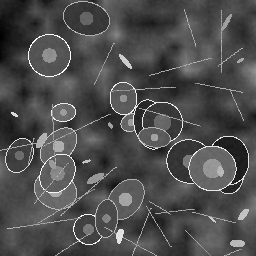
Forward-Model Mismatch Cases
- The widefield fallback applies optical Gaussian blur, but SEM image formation involves electron-sample interaction (secondary electron yield depends on surface topography and composition) — the contrast mechanism is fundamentally different from optical fluorescence
- SEM contrast (SE and BSE signals) depends on accelerating voltage, material Z-number, surface tilt, and detector geometry — the widefield PSF convolution model cannot capture these electron-matter interaction physics
How to Correct the Mismatch
- Use the SEM operator that models the electron probe profile (sub-nm spot) and secondary/backscattered electron yield as a function of local surface topography and composition
- Include the interaction volume (Monte Carlo electron trajectory simulation), detector angular acceptance, and signal mixing between SE (topography) and BSE (composition) channels
Experimental Setup — Signal Chain

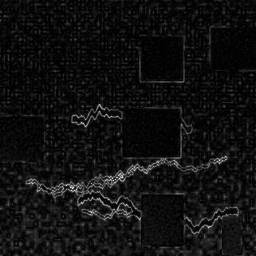
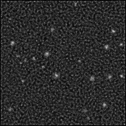
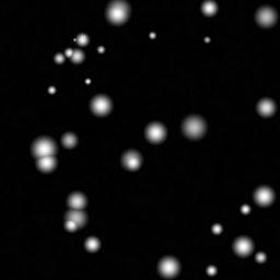
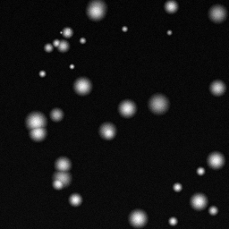
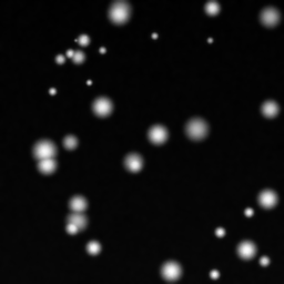
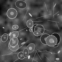
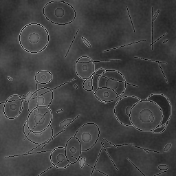
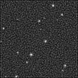
Reconstruction Gallery — 4 Scenes × 3 Scenarios
Method: CPU_baseline | Mismatch: nominal (nominal=True, perturbed=False)
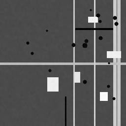
Ground Truth

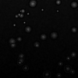
Measurement

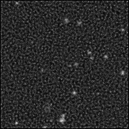
Reconstruction
Ground Truth

Measurement
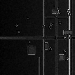
Reconstruction
Ground Truth
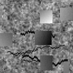
Measurement (perturbed)
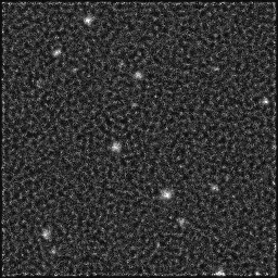
Reconstruction


Mean PSNR Across All Scenes
Per-scene PSNR breakdown (4 scenes)
| Scene | I (PSNR) | I (SSIM) | II (PSNR) | II (SSIM) | III (PSNR) | III (SSIM) |
|---|---|---|---|---|---|---|
| scene_00 | 27.207707576015594 | 0.9294173230245113 | 9.87621406035924 | 0.15544546946127621 | 11.930071915823044 | 0.07164574915011365 |
| scene_01 | 28.196073532215188 | 0.9224614043250083 | 7.154560564346867 | 0.09150285540748944 | 9.118605033501924 | 0.049539999208181425 |
| scene_02 | 35.4163412021651 | 0.7281297008299827 | 18.08344905811649 | 0.5046347770228695 | 13.44839939845765 | 0.009466454033365426 |
| scene_03 | 23.3890361189313 | 0.8550307007561923 | 15.028289192835638 | 0.18117373205865303 | 13.858955008713668 | 0.06355400138100081 |
| Mean | 28.552289607331794 | 0.8587597822339237 | 12.535628218914558 | 0.23318920848757207 | 12.089007839124072 | 0.04855155094316533 |
Experimental Setup
Key References
- Goldstein et al., 'Scanning Electron Microscopy and X-ray Microanalysis', Springer (2018)
Canonical Datasets
- SEM Dataset for Nanomaterial Segmentation (Aversa et al.)
- NIST SEM calibration images
Spec DAG — Forward Model Pipeline
P(e⁻ beam) → C(probe) → D(g, η₁)
Mismatch Parameters
| Symbol | Parameter | Description | Nominal | Perturbed |
|---|---|---|---|---|
| ΔE | beam_energy | Beam energy error (keV) | 0 | 0.1 |
| ΔA_s | stigmatism | Astigmatism (nm) | 0 | 5.0 |
| ΔWD | working_distance | Working distance error (mm) | 0 | 0.1 |
Credits System
Spec Primitives Reference (11 primitives)
Free-space or medium propagation kernel (Fresnel, Rayleigh-Sommerfeld).
Spatial or spatio-temporal amplitude modulation (coded aperture, SLM pattern).
Geometric projection operator (Radon transform, fan-beam, cone-beam).
Sampling in the Fourier / k-space domain (MRI, ptychography).
Shift-invariant convolution with a point-spread function (PSF).
Summation along a physical dimension (spectral, temporal, angular).
Sensor readout with gain g and noise model η (Gaussian, Poisson, mixed).
Patterned illumination (block, Hadamard, random) applied to the scene.
Spectral dispersion element (prism, grating) with shift α and aperture a.
Sample or gantry rotation (CT, electron tomography).
Spectral filter or monochromator selecting a wavelength band.