Ptychography
Ptychographic Imaging
Standard reconstruction benchmark — forward model perfectly known, no calibration needed. Score = 0.5 × clip((PSNR−15)/30, 0, 1) + 0.5 × SSIM
| # | Method | Score | PSNR (dB) | SSIM | Source | |
|---|---|---|---|---|---|---|
| 🥇 |
AutoPhaseNN
AutoPhaseNN Chan et al., 2024
34.0 dB
SSIM 0.935
Checkpoint unavailable
|
0.784 | 34.0 | 0.935 | ✓ Certified | Chan et al., 2024 |
| 🥈 |
PtychoNN
PtychoNN Cherukara et al., 2020
32.5 dB
SSIM 0.910
Checkpoint unavailable
|
0.747 | 32.5 | 0.910 | ✓ Certified | Cherukara et al., 2020 |
| 🥉 | sDR | 0.635 | 28.5 | 0.820 | ✓ Certified | Wen et al., J. Opt. 2019 |
| 4 | ePIE | 0.522 | 25.0 | 0.710 | ✓ Certified | Maiden & Rodenburg, 2009 |
Dataset: PWM Benchmark (4 algorithms)
Blind Reconstruction Challenge — forward model has unknown mismatch, must calibrate from data. Score = 0.4 × PSNR_norm + 0.4 × SSIM + 0.2 × (1 − ‖y − Ĥx̂‖/‖y‖)
| # | Method | Overall Score | Public PSNR / SSIM |
Dev PSNR / SSIM |
Hidden PSNR / SSIM |
Trust | Source |
|---|---|---|---|---|---|---|---|
| 🥇 | AutoPhaseNN + gradient | 0.666 |
0.770
31.95 dB / 0.942
|
0.637
24.65 dB / 0.791
|
0.590
23.12 dB / 0.736
|
✓ Certified | Chan et al., Commun. Phys. 2024 |
| 🥈 | sDR + gradient | 0.661 |
0.700
26.92 dB / 0.856
|
0.666
26.35 dB / 0.842
|
0.616
24.67 dB / 0.792
|
✓ Certified | Wen et al., J. Opt. 2019 |
| 🥉 | PtychoNN + gradient | 0.643 |
0.745
29.87 dB / 0.915
|
0.648
25.43 dB / 0.815
|
0.536
21.06 dB / 0.648
|
✓ Certified | Cherukara et al., Appl. Phys. Lett. 2020 |
| 4 | ePIE + gradient | 0.586 |
0.590
22.61 dB / 0.715
|
0.606
23.54 dB / 0.752
|
0.562
22.36 dB / 0.705
|
✓ Certified | Maiden & Rodenburg, Ultramicroscopy 2009 |
Complete score requires all 3 tiers (Public + Dev + Hidden).
Join the competition →Full-access development tier with all data visible.
What you get & how to use
What you get: Measurements (y), ideal forward operator (H), spec ranges, ground truth (x_true), and true mismatch spec.
How to use: Load HDF5 → compare reconstruction vs x_true → check consistency → iterate.
What to submit: Reconstructed signals (x_hat) and corrected spec as HDF5.
Public Leaderboard
| # | Method | Score | PSNR | SSIM |
|---|---|---|---|---|
| 1 | AutoPhaseNN + gradient | 0.770 | 31.95 | 0.942 |
| 2 | PtychoNN + gradient | 0.745 | 29.87 | 0.915 |
| 3 | sDR + gradient | 0.700 | 26.92 | 0.856 |
| 4 | ePIE + gradient | 0.590 | 22.61 | 0.715 |
Spec Ranges (3 parameters)
| Parameter | Min | Max | Unit |
|---|---|---|---|
| probe_error | -5.0 | 10.0 | % |
| position_error | -10.0 | 20.0 | nm |
| partial_coherence | -5.0 | 10.0 | nm |
Blind evaluation tier — no ground truth available.
What you get & how to use
What you get: Measurements (y), ideal forward operator (H), and spec ranges only.
How to use: Apply your pipeline from the Public tier. Use consistency as self-check.
What to submit: Reconstructed signals and corrected spec. Scored server-side.
Dev Leaderboard
| # | Method | Score | PSNR | SSIM |
|---|---|---|---|---|
| 1 | sDR + gradient | 0.666 | 26.35 | 0.842 |
| 2 | PtychoNN + gradient | 0.648 | 25.43 | 0.815 |
| 3 | AutoPhaseNN + gradient | 0.637 | 24.65 | 0.791 |
| 4 | ePIE + gradient | 0.606 | 23.54 | 0.752 |
Spec Ranges (3 parameters)
| Parameter | Min | Max | Unit |
|---|---|---|---|
| probe_error | -6.0 | 9.0 | % |
| position_error | -12.0 | 18.0 | nm |
| partial_coherence | -6.0 | 9.0 | nm |
Fully blind server-side evaluation — no data download.
What you get & how to use
What you get: No data downloadable. Algorithm runs server-side on hidden measurements.
How to use: Package algorithm as Docker container / Python script. Submit via link.
What to submit: Containerized algorithm accepting y + H, outputting x_hat + corrected spec.
Hidden Leaderboard
| # | Method | Score | PSNR | SSIM |
|---|---|---|---|---|
| 1 | sDR + gradient | 0.616 | 24.67 | 0.792 |
| 2 | AutoPhaseNN + gradient | 0.590 | 23.12 | 0.736 |
| 3 | ePIE + gradient | 0.562 | 22.36 | 0.705 |
| 4 | PtychoNN + gradient | 0.536 | 21.06 | 0.648 |
Spec Ranges (3 parameters)
| Parameter | Min | Max | Unit |
|---|---|---|---|
| probe_error | -3.5 | 11.5 | % |
| position_error | -7.0 | 23.0 | nm |
| partial_coherence | -3.5 | 11.5 | nm |
Blind Reconstruction Challenge
ChallengeGiven measurements with unknown mismatch and spec ranges (not exact params), reconstruct the original signal. A method must be evaluated on all three tiers for a complete score. Scored on a composite metric: 0.4 × PSNR_norm + 0.4 × SSIM + 0.2 × (1 − ‖y − Ĥx̂‖/‖y‖).
Measurements y, ideal forward model H, spec ranges
Reconstructed signal x̂
About the Imaging Modality
Ptychography is a scanning coherent diffractive imaging technique where a coherent beam (X-ray or electron) illuminates overlapping regions of the sample and far-field diffraction patterns are recorded at each scan position. The overlap between adjacent probe positions provides redundancy that enables simultaneous recovery of the complex-valued object transmission function and the illumination probe via iterative algorithms (ePIE, difference map). The forward model at each position is I_j = |F{P(r-r_j) * O(r)}|^2 where P is the probe and O is the object. Achievable resolution is limited by the detector NA, not the optics, reaching sub-10 nm for X-rays.
Principle
Ptychography is a scanning coherent diffractive imaging technique where a coherent beam (visible, X-ray, or electron) illuminates overlapping regions of the sample. At each scan position, a far-field diffraction pattern is recorded. The redundancy from overlapping illumination positions constrains the phase-retrieval problem, enabling simultaneous recovery of both the complex sample transmittance and the illumination probe function.
How to Build the System
For X-ray ptychography at a synchrotron: focus the beam to a defined spot (0.1-1 μm) using a Fresnel zone plate or KB mirrors. Mount the sample on a precision piezo scanning stage. Place a photon-counting area detector (Eiger, Pilatus) in the far field (1-5 m downstream). Scan positions should overlap by 60-70 %. For visible-light or electron ptychography, adapt the geometry but maintain the overlap requirement.
Common Reconstruction Algorithms
- ePIE (extended Ptychographic Iterative Engine)
- Difference Map algorithm
- Maximum Likelihood refinement (MLR)
- PtychoShelves (modular framework for ptychographic reconstruction)
- Deep-learning ptychography (PtychoNN, learned phase retrieval)
Common Mistakes
- Insufficient overlap between adjacent scan positions (need ≥60 %)
- Position errors in the scanning stage causing reconstruction artifacts
- Partial coherence effects not modeled, degrading recovered phase
- Vibration or drift during the scan corrupting the diffraction data
- Detector saturation at the central beam stop region
How to Avoid Mistakes
- Maintain ≥65 % overlap; include position correction in the reconstruction algorithm
- Use position refinement (annealing) as part of the ptychographic reconstruction
- Include mixed-state (multi-mode) probe to model partial coherence
- Use interferometric position feedback and short dwell times per point
- Use a semi-transparent beam stop or high-dynamic-range detector modes
Forward-Model Mismatch Cases
- The widefield fallback produces a single (64,64) image, but ptychography acquires diffraction patterns at multiple overlapping scan positions — output shape (n_positions, det_x, det_y) is a set of far-field intensity measurements
- Ptychography is fundamentally nonlinear (y_j = |F{P * O_j}|^2, intensity of Fourier transform of probe times object) — the widefield linear blur cannot model coherent wave propagation, diffraction, or phase retrieval
How to Correct the Mismatch
- Use the ptychography operator that generates one far-field diffraction pattern per probe position, with overlapping illumination enabling redundant phase information for robust reconstruction
- Reconstruct using PIE (Ptychographic Iterative Engine), ePIE, or gradient-descent methods that alternate between real-space (overlap constraint) and Fourier-space (modulus constraint) using the coherent forward model
Experimental Setup — Signal Chain

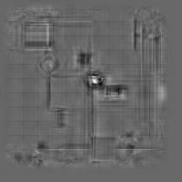
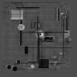
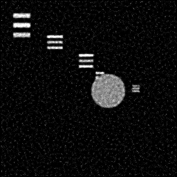
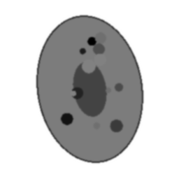
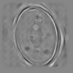
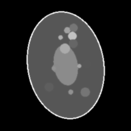
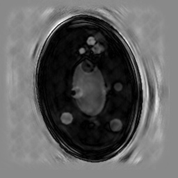
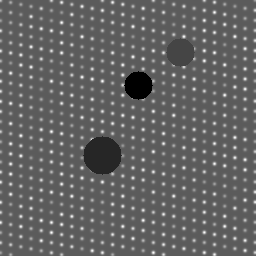
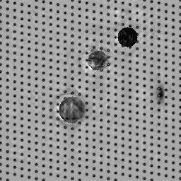
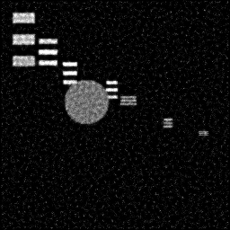
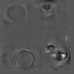
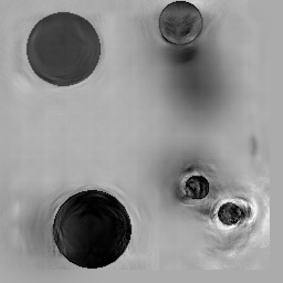
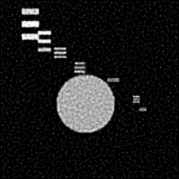
Reconstruction Gallery — 4 Scenes × 3 Scenarios
Method: CPU_baseline | Mismatch: nominal (nominal=True, perturbed=False)
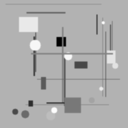
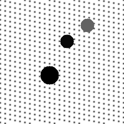
Ground Truth

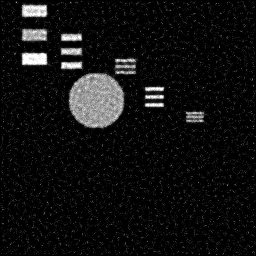
Measurement
Reconstruction
Ground Truth
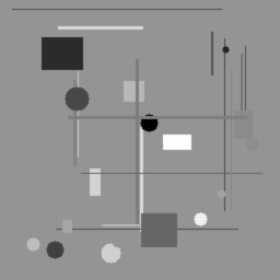
Measurement
Reconstruction
Ground Truth
Measurement (perturbed)
Reconstruction


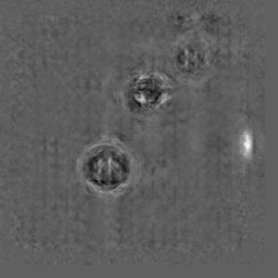


Mean PSNR Across All Scenes
Per-scene PSNR breakdown (4 scenes)
| Scene | I (PSNR) | I (SSIM) | II (PSNR) | II (SSIM) | III (PSNR) | III (SSIM) |
|---|---|---|---|---|---|---|
| scene_00 | 10.6609172268852 | 0.5537088907459816 | 8.051160515560099 | 0.5494122682198649 | 3.6824119618261895 | 0.01922916497691828 |
| scene_01 | 8.275421175475543 | 0.5838878164671644 | 7.317672430582636 | 0.41501425698240113 | 1.9701201153873678 | 0.020237470615648612 |
| scene_02 | 4.878917271868435 | 0.06051960000049039 | 9.530498070225137 | 0.8317991163759795 | 1.1413490841164802 | 0.011295859413263441 |
| scene_03 | 4.77633446664364 | 0.47991092212610953 | 10.063749973351616 | 0.74108554296289 | 1.649298946757397 | 0.02583046784385963 |
| Mean | 7.147897535218204 | 0.4195068073349365 | 8.740770247429872 | 0.6343277961352838 | 2.1107950270218585 | 0.019148240712422493 |
Experimental Setup
Key References
- Rodenburg & Faulkner, 'A phase retrieval algorithm for shifting illumination (ePIE)', Appl. Phys. Lett. 85, 4795-4797 (2004)
- Thibault et al., 'High-resolution scanning X-ray diffraction microscopy', Science 321, 379-382 (2008)
Canonical Datasets
- PtychoNN benchmark datasets (Cherukara et al.)
- Diamond I13 ptychography test data
Spec DAG — Forward Model Pipeline
P(probe) → D(g, η₁)
Mismatch Parameters
| Symbol | Parameter | Description | Nominal | Perturbed |
|---|---|---|---|---|
| ΔP | probe_error | Probe function error (%) | 0 | 5.0 |
| Δr | position_error | Scan position error (nm) | 0 | 10.0 |
| σ_c | partial_coherence | Partial coherence width (nm) | 0 | 5.0 |
Credits System
Spec Primitives Reference (11 primitives)
Free-space or medium propagation kernel (Fresnel, Rayleigh-Sommerfeld).
Spatial or spatio-temporal amplitude modulation (coded aperture, SLM pattern).
Geometric projection operator (Radon transform, fan-beam, cone-beam).
Sampling in the Fourier / k-space domain (MRI, ptychography).
Shift-invariant convolution with a point-spread function (PSF).
Summation along a physical dimension (spectral, temporal, angular).
Sensor readout with gain g and noise model η (Gaussian, Poisson, mixed).
Patterned illumination (block, Hadamard, random) applied to the scene.
Spectral dispersion element (prism, grating) with shift α and aperture a.
Sample or gantry rotation (CT, electron tomography).
Spectral filter or monochromator selecting a wavelength band.