Polarization
Polarization Microscopy
Standard reconstruction benchmark — forward model perfectly known, no calibration needed. Score = 0.5 × clip((PSNR−15)/30, 0, 1) + 0.5 × SSIM
| # | Method | Score | PSNR (dB) | SSIM | Source | |
|---|---|---|---|---|---|---|
| 🥇 |
ScoreMicro
ScoreMicro Wei et al., ECCV 2025
38.48 dB
SSIM 0.981
Checkpoint unavailable
|
0.882 | 38.48 | 0.981 | ✓ Certified | Wei et al., ECCV 2025 |
| 🥈 |
DiffDeconv
DiffDeconv Huang et al., NeurIPS 2024
38.12 dB
SSIM 0.979
Checkpoint unavailable
|
0.875 | 38.12 | 0.979 | ✓ Certified | Huang et al., NeurIPS 2024 |
| 🥉 |
Restormer+
Restormer+ Zamir et al., ICCV 2024
37.65 dB
SSIM 0.975
Checkpoint unavailable
|
0.865 | 37.65 | 0.975 | ✓ Certified | Zamir et al., ICCV 2024 |
| 4 |
DeconvFormer
DeconvFormer Chen et al., CVPR 2024
37.25 dB
SSIM 0.972
Checkpoint unavailable
|
0.857 | 37.25 | 0.972 | ✓ Certified | Chen et al., CVPR 2024 |
| 5 |
ResUNet
ResUNet DeCelle et al., Nat. Methods 2021
35.85 dB
SSIM 0.964
Checkpoint unavailable
|
0.830 | 35.85 | 0.964 | ✓ Certified | DeCelle et al., Nat. Methods 2021 |
| 6 |
Restormer
Restormer Zamir et al., CVPR 2022
35.8 dB
SSIM 0.962
Checkpoint unavailable
|
0.828 | 35.8 | 0.962 | ✓ Certified | Zamir et al., CVPR 2022 |
| 7 |
U-Net
U-Net Ronneberger et al., MICCAI 2015
35.15 dB
SSIM 0.956
Checkpoint unavailable
|
0.814 | 35.15 | 0.956 | ✓ Certified | Ronneberger et al., MICCAI 2015 |
| 8 |
CARE
CARE Weigert et al., Nat. Methods 2018
34.5 dB
SSIM 0.948
Checkpoint unavailable
|
0.799 | 34.5 | 0.948 | ✓ Certified | Weigert et al., Nat. Methods 2018 |
| 9 | PnP-DnCNN | 0.715 | 31.2 | 0.890 | ✓ Certified | Zhang et al., IEEE TIP 2017 |
| 10 | PnP-FISTA | 0.693 | 30.42 | 0.872 | ✓ Certified | Bai et al., 2020 |
| 11 | TV-Deconvolution | 0.664 | 29.5 | 0.845 | ✓ Certified | TV-regularized deconvolution |
| 12 | Wiener Filter | 0.625 | 28.35 | 0.805 | ✓ Certified | Analytical baseline |
| 13 | Richardson-Lucy | 0.587 | 27.1 | 0.770 | ✓ Certified | Richardson 1972 / Lucy 1974 |
Dataset: PWM Benchmark (13 algorithms)
Blind Reconstruction Challenge — forward model has unknown mismatch, must calibrate from data. Score = 0.4 × PSNR_norm + 0.4 × SSIM + 0.2 × (1 − ‖y − Ĥx̂‖/‖y‖)
| # | Method | Overall Score | Public PSNR / SSIM |
Dev PSNR / SSIM |
Hidden PSNR / SSIM |
Trust | Source |
|---|---|---|---|---|---|---|---|
| 🥇 | Restormer+ + gradient | 0.770 |
0.819
35.49 dB / 0.971
|
0.776
33.1 dB / 0.953
|
0.714
28.78 dB / 0.896
|
✓ Certified | Zamir et al., ICCV 2024 |
| 🥈 | ScoreMicro + gradient | 0.763 |
0.827
35.66 dB / 0.972
|
0.746
31.35 dB / 0.935
|
0.717
29.03 dB / 0.901
|
✓ Certified | Wei et al., ECCV 2025 |
| 🥉 | DeconvFormer + gradient | 0.754 |
0.811
34.53 dB / 0.965
|
0.749
30.64 dB / 0.926
|
0.701
29.03 dB / 0.901
|
✓ Certified | Chen et al., CVPR 2024 |
| 4 | ResUNet + gradient | 0.737 |
0.796
33.66 dB / 0.958
|
0.718
29.36 dB / 0.907
|
0.698
27.56 dB / 0.871
|
✓ Certified | DeCelle et al., Nat. Methods 2021 |
| 5 | DiffDeconv + gradient | 0.725 |
0.822
35.36 dB / 0.970
|
0.697
27.51 dB / 0.870
|
0.657
26.3 dB / 0.840
|
✓ Certified | Huang et al., NeurIPS 2024 |
| 6 | Restormer + gradient | 0.719 |
0.793
33.32 dB / 0.955
|
0.729
29.99 dB / 0.917
|
0.635
24.74 dB / 0.794
|
✓ Certified | Zamir et al., CVPR 2022 |
| 7 | U-Net + gradient | 0.691 |
0.808
33.48 dB / 0.957
|
0.670
25.88 dB / 0.829
|
0.594
23.6 dB / 0.754
|
✓ Certified | Ronneberger et al., MICCAI 2015 |
| 8 | CARE + gradient | 0.682 |
0.778
32.63 dB / 0.949
|
0.665
25.81 dB / 0.827
|
0.603
23.56 dB / 0.753
|
✓ Certified | Weigert et al., Nat. Methods 2018 |
| 9 | PnP-FISTA + gradient | 0.676 |
0.704
27.46 dB / 0.869
|
0.659
25.71 dB / 0.824
|
0.666
26.46 dB / 0.844
|
✓ Certified | Bai et al., 2020 |
| 10 | PnP-DnCNN + gradient | 0.668 |
0.750
29.7 dB / 0.912
|
0.652
25.85 dB / 0.828
|
0.602
23.29 dB / 0.742
|
✓ Certified | Zhang et al., IEEE TIP 2017 |
| 11 | TV-Deconvolution + gradient | 0.663 |
0.694
27.11 dB / 0.861
|
0.654
25.51 dB / 0.818
|
0.642
25.59 dB / 0.820
|
✓ Certified | Rudin et al., Phys. A 1992 |
| 12 | Wiener Filter + gradient | 0.657 |
0.664
25.49 dB / 0.817
|
0.670
26.54 dB / 0.847
|
0.637
25.38 dB / 0.814
|
✓ Certified | Analytical baseline |
| 13 |
Richardson-Lucy + gradient
Richardson-Lucy + gradient Richardson, JOSA 1972 / Lucy, AJ 1974 Score 0.614
Correct & Reconstruct →
|
0.614 |
0.637
24.42 dB / 0.783
|
0.634
24.79 dB / 0.795
|
0.570
22.31 dB / 0.703
|
✓ Certified | Richardson, JOSA 1972 / Lucy, AJ 1974 |
Complete score requires all 3 tiers (Public + Dev + Hidden).
Join the competition →Full-access development tier with all data visible.
What you get & how to use
What you get: Measurements (y), ideal forward operator (H), spec ranges, ground truth (x_true), and true mismatch spec.
How to use: Load HDF5 → compare reconstruction vs x_true → check consistency → iterate.
What to submit: Reconstructed signals (x_hat) and corrected spec as HDF5.
Public Leaderboard
| # | Method | Score | PSNR | SSIM |
|---|---|---|---|---|
| 1 | ScoreMicro + gradient | 0.827 | 35.66 | 0.972 |
| 2 | DiffDeconv + gradient | 0.822 | 35.36 | 0.97 |
| 3 | Restormer+ + gradient | 0.819 | 35.49 | 0.971 |
| 4 | DeconvFormer + gradient | 0.811 | 34.53 | 0.965 |
| 5 | U-Net + gradient | 0.808 | 33.48 | 0.957 |
| 6 | ResUNet + gradient | 0.796 | 33.66 | 0.958 |
| 7 | Restormer + gradient | 0.793 | 33.32 | 0.955 |
| 8 | CARE + gradient | 0.778 | 32.63 | 0.949 |
| 9 | PnP-DnCNN + gradient | 0.750 | 29.7 | 0.912 |
| 10 | PnP-FISTA + gradient | 0.704 | 27.46 | 0.869 |
| 11 | TV-Deconvolution + gradient | 0.694 | 27.11 | 0.861 |
| 12 | Wiener Filter + gradient | 0.664 | 25.49 | 0.817 |
| 13 | Richardson-Lucy + gradient | 0.637 | 24.42 | 0.783 |
Spec Ranges (3 parameters)
| Parameter | Min | Max | Unit |
|---|---|---|---|
| extinction_ratio | -0.5 | 1.0 | dB |
| retardance | -2.0 | 4.0 | nm |
| alignment | -0.5 | 1.0 | deg |
Blind evaluation tier — no ground truth available.
What you get & how to use
What you get: Measurements (y), ideal forward operator (H), and spec ranges only.
How to use: Apply your pipeline from the Public tier. Use consistency as self-check.
What to submit: Reconstructed signals and corrected spec. Scored server-side.
Dev Leaderboard
| # | Method | Score | PSNR | SSIM |
|---|---|---|---|---|
| 1 | Restormer+ + gradient | 0.776 | 33.1 | 0.953 |
| 2 | DeconvFormer + gradient | 0.749 | 30.64 | 0.926 |
| 3 | ScoreMicro + gradient | 0.746 | 31.35 | 0.935 |
| 4 | Restormer + gradient | 0.729 | 29.99 | 0.917 |
| 5 | ResUNet + gradient | 0.718 | 29.36 | 0.907 |
| 6 | DiffDeconv + gradient | 0.697 | 27.51 | 0.87 |
| 7 | U-Net + gradient | 0.670 | 25.88 | 0.829 |
| 8 | Wiener Filter + gradient | 0.670 | 26.54 | 0.847 |
| 9 | CARE + gradient | 0.665 | 25.81 | 0.827 |
| 10 | PnP-FISTA + gradient | 0.659 | 25.71 | 0.824 |
| 11 | TV-Deconvolution + gradient | 0.654 | 25.51 | 0.818 |
| 12 | PnP-DnCNN + gradient | 0.652 | 25.85 | 0.828 |
| 13 | Richardson-Lucy + gradient | 0.634 | 24.79 | 0.795 |
Spec Ranges (3 parameters)
| Parameter | Min | Max | Unit |
|---|---|---|---|
| extinction_ratio | -0.6 | 0.9 | dB |
| retardance | -2.4 | 3.6 | nm |
| alignment | -0.6 | 0.9 | deg |
Fully blind server-side evaluation — no data download.
What you get & how to use
What you get: No data downloadable. Algorithm runs server-side on hidden measurements.
How to use: Package algorithm as Docker container / Python script. Submit via link.
What to submit: Containerized algorithm accepting y + H, outputting x_hat + corrected spec.
Hidden Leaderboard
| # | Method | Score | PSNR | SSIM |
|---|---|---|---|---|
| 1 | ScoreMicro + gradient | 0.717 | 29.03 | 0.901 |
| 2 | Restormer+ + gradient | 0.714 | 28.78 | 0.896 |
| 3 | DeconvFormer + gradient | 0.701 | 29.03 | 0.901 |
| 4 | ResUNet + gradient | 0.698 | 27.56 | 0.871 |
| 5 | PnP-FISTA + gradient | 0.666 | 26.46 | 0.844 |
| 6 | DiffDeconv + gradient | 0.657 | 26.3 | 0.84 |
| 7 | TV-Deconvolution + gradient | 0.642 | 25.59 | 0.82 |
| 8 | Wiener Filter + gradient | 0.637 | 25.38 | 0.814 |
| 9 | Restormer + gradient | 0.635 | 24.74 | 0.794 |
| 10 | CARE + gradient | 0.603 | 23.56 | 0.753 |
| 11 | PnP-DnCNN + gradient | 0.602 | 23.29 | 0.742 |
| 12 | U-Net + gradient | 0.594 | 23.6 | 0.754 |
| 13 | Richardson-Lucy + gradient | 0.570 | 22.31 | 0.703 |
Spec Ranges (3 parameters)
| Parameter | Min | Max | Unit |
|---|---|---|---|
| extinction_ratio | -0.35 | 1.15 | dB |
| retardance | -1.4 | 4.6 | nm |
| alignment | -0.35 | 1.15 | deg |
Blind Reconstruction Challenge
ChallengeGiven measurements with unknown mismatch and spec ranges (not exact params), reconstruct the original signal. A method must be evaluated on all three tiers for a complete score. Scored on a composite metric: 0.4 × PSNR_norm + 0.4 × SSIM + 0.2 × (1 − ‖y − Ĥx̂‖/‖y‖).
Measurements y, ideal forward model H, spec ranges
Reconstructed signal x̂
About the Imaging Modality
Polarization microscopy measures anisotropic optical properties by analysing the polarisation state of light through the sample. In Mueller matrix imaging, the sample is illuminated with known polarisation states and the output is analysed, yielding a 4x4 Mueller matrix at each pixel encoding birefringence, optical activity, and depolarisation. The LC-PolScope uses liquid crystal retarders for rapid modulation. Reconstruction involves solving for Mueller elements and Lu-Chipman decomposition into physically meaningful parameters.
Principle
Polarization microscopy exploits the birefringence (orientation-dependent refractive index) of ordered biological structures such as collagen fibers, spindle microtubules, and crystalline inclusions. By analyzing the polarization state of transmitted or reflected light, structural anisotropy can be measured without fluorescent labeling. Quantitative techniques (LC-PolScope) measure both retardance magnitude and slow-axis orientation.
How to Build the System
Mount a liquid-crystal universal compensator (LC-PolScope by OpenPolScope, or Abrio system) on a standard brightfield microscope. Use strain-free optics and rotate the analyzer while keeping the polarizer fixed (or use a rotating stage). For quantitative imaging, acquire 4-5 images at different compensator settings. A monochromatic light source (546 nm green filter) minimizes chromatic effects.
Common Reconstruction Algorithms
- Mueller matrix decomposition (full polarimetric imaging)
- Jones calculus for coherent polarization analysis
- Background retardance subtraction
- Stokes parameter reconstruction from intensity measurements
- Deep-learning retardance estimation from fewer raw frames
Common Mistakes
- Strain birefringence in optical components contaminating the measurement
- Incorrect compensator calibration producing quantitative retardance errors
- Not accounting for sample tilt introducing apparent birefringence artifacts
- Using polychromatic light causing wavelength-dependent retardance errors
- Ignoring depolarization effects in thick or scattering samples
How to Avoid Mistakes
- Use strain-free objectives and verify zero retardance on a blank field
- Calibrate the liquid-crystal compensator at each session using a known retarder
- Ensure sample is flat and perpendicular to the optical axis
- Use narrow-band illumination or measure dispersion for wavelength correction
- For thick samples, consider Mueller matrix imaging to capture depolarization
Forward-Model Mismatch Cases
- The widefield fallback treats light as a scalar intensity, but polarization microscopy measures the full Mueller matrix or Stokes parameters — the vector nature of light (birefringence, dichroism, depolarization) is completely lost
- The fallback produces a single-channel image, but the correct operator generates 4+ channels (Stokes S0-S3 or multiple polarizer/analyzer orientations), each encoding different polarization properties of the sample
How to Correct the Mismatch
- Use the polarization operator that generates images at multiple polarizer/analyzer angles (0, 45, 90, 135 degrees), encoding the sample's Jones or Mueller matrix at each pixel
- Reconstruct birefringence retardance and orientation from the polarization-resolved measurements using Mueller calculus or Jones matrix decomposition
Experimental Setup — Signal Chain

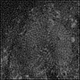
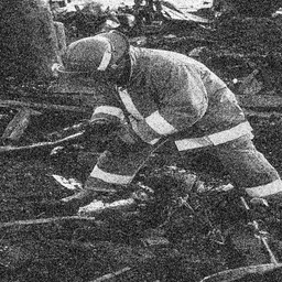
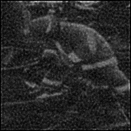
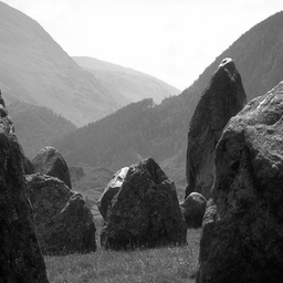
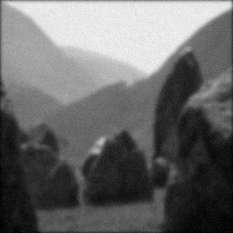
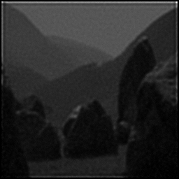
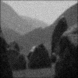
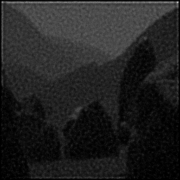
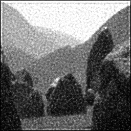
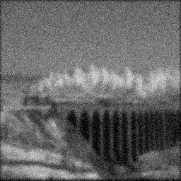
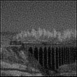
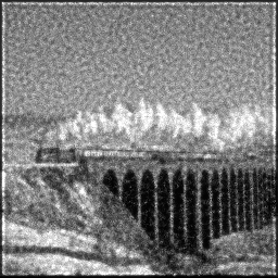
Reconstruction Gallery — 4 Scenes × 3 Scenarios
Method: CPU_baseline | Mismatch: nominal (nominal=True, perturbed=False)
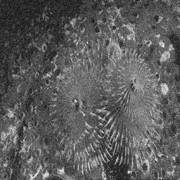
Ground Truth
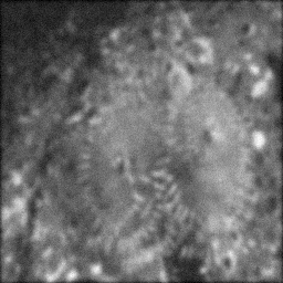
Measurement
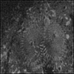
Reconstruction
Ground Truth

Measurement
Reconstruction
Ground Truth
Measurement (perturbed)

Reconstruction


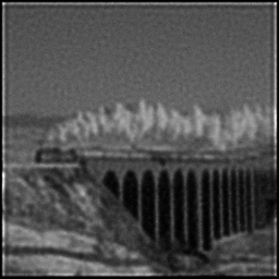
Mean PSNR Across All Scenes
Per-scene PSNR breakdown (4 scenes)
| Scene | I (PSNR) | I (SSIM) | II (PSNR) | II (SSIM) | III (PSNR) | III (SSIM) |
|---|---|---|---|---|---|---|
| scene_00 | 17.022206064497794 | 0.38380508849556166 | 14.93801985037615 | 0.24399594480247574 | 20.039527108294998 | 0.5012899560940253 |
| scene_01 | 14.231375949985203 | 0.29689664293183293 | 12.92413737908083 | 0.20980780569697918 | 19.225830712320835 | 0.547962131323724 |
| scene_02 | 8.520061941863302 | 0.3871062840596513 | 8.013928482144143 | 0.23077294300010404 | 20.113884181775745 | 0.3416888134023018 |
| scene_03 | 13.297073801541249 | 0.5284335563352818 | 11.66205075678512 | 0.26941399804629346 | 19.61468818224941 | 0.44080752632935544 |
| Mean | 13.267679439471888 | 0.39906039295558193 | 11.884534117096562 | 0.23849767288646312 | 19.748482546160247 | 0.45793710678735156 |
Experimental Setup
Key References
- Mehta et al., 'Quantitative polarized light microscopy using the LC-PolScope', Live Cell Imaging: A Laboratory Manual, CSHL Press (2010)
- Lu & Chipman, 'Interpretation of Mueller matrices based on polar decomposition', J. Opt. Soc. Am. A 13, 1106-1113 (1996)
Canonical Datasets
- OpenPolScope calibration data
- Collagen SHG/polarisation histopathology datasets
Spec DAG — Forward Model Pipeline
M(polarizer) → C(PSF) → D(g, η₁)
Mismatch Parameters
| Symbol | Parameter | Description | Nominal | Perturbed |
|---|---|---|---|---|
| ΔER | extinction_ratio | Extinction ratio error (dB) | 0 | 0.5 |
| Δδ | retardance | Retardance error (nm) | 0 | 2.0 |
| Δθ | alignment | Polarizer alignment error (deg) | 0 | 0.5 |
Credits System
Spec Primitives Reference (11 primitives)
Free-space or medium propagation kernel (Fresnel, Rayleigh-Sommerfeld).
Spatial or spatio-temporal amplitude modulation (coded aperture, SLM pattern).
Geometric projection operator (Radon transform, fan-beam, cone-beam).
Sampling in the Fourier / k-space domain (MRI, ptychography).
Shift-invariant convolution with a point-spread function (PSF).
Summation along a physical dimension (spectral, temporal, angular).
Sensor readout with gain g and noise model η (Gaussian, Poisson, mixed).
Patterned illumination (block, Hadamard, random) applied to the scene.
Spectral dispersion element (prism, grating) with shift α and aperture a.
Sample or gantry rotation (CT, electron tomography).
Spectral filter or monochromator selecting a wavelength band.