Photoacoustic
Photoacoustic Imaging
Standard reconstruction benchmark — forward model perfectly known, no calibration needed. Score = 0.5 × clip((PSNR−15)/30, 0, 1) + 0.5 × SSIM
| # | Method | Score | PSNR (dB) | SSIM | Source | |
|---|---|---|---|---|---|---|
| 🥇 |
PAT-Former
PAT-Former PAT reconstruction transformer, 2024
33.5 dB
SSIM 0.920
Checkpoint unavailable
|
0.768 | 33.5 | 0.920 | ✓ Certified | PAT reconstruction transformer, 2024 |
| 🥈 |
Deep-PAI
Deep-PAI Hauptmann et al., IEEE TMI 2018
31.5 dB
SSIM 0.890
Checkpoint unavailable
|
0.720 | 31.5 | 0.890 | ✓ Certified | Hauptmann et al., IEEE TMI 2018 |
| 🥉 | PnP-ADMM | 0.595 | 27.0 | 0.790 | ✓ Certified | Goudarzi et al., 2020 |
| 4 | Universal Back-Proj | 0.462 | 23.5 | 0.640 | ✓ Certified | Xu & Wang, Phys. Rev. E 2005 |
Dataset: PWM Benchmark (4 algorithms)
Blind Reconstruction Challenge — forward model has unknown mismatch, must calibrate from data. Score = 0.4 × PSNR_norm + 0.4 × SSIM + 0.2 × (1 − ‖y − Ĥx̂‖/‖y‖)
| # | Method | Overall Score | Public PSNR / SSIM |
Dev PSNR / SSIM |
Hidden PSNR / SSIM |
Trust | Source |
|---|---|---|---|---|---|---|---|
| 🥇 | PAT-Former + gradient | 0.682 |
0.764
31.37 dB / 0.935
|
0.680
27.12 dB / 0.861
|
0.601
23.19 dB / 0.738
|
✓ Certified | PAT reconstruction transformer, 2024 |
| 🥈 | Deep-PAI + gradient | 0.602 |
0.730
29.1 dB / 0.902
|
0.557
21.58 dB / 0.672
|
0.520
20.55 dB / 0.625
|
✓ Certified | Hauptmann et al., IEEE TMI 2018 |
| 🥉 | Universal Back-Proj + gradient | 0.551 |
0.542
20.8 dB / 0.636
|
0.566
22.14 dB / 0.696
|
0.545
21.58 dB / 0.672
|
✓ Certified | Xu & Wang, Phys. Rev. E 2005 |
| 4 | PnP-ADMM + gradient | 0.521 |
0.641
24.74 dB / 0.794
|
0.513
20.33 dB / 0.614
|
0.410
17.4 dB / 0.470
|
✓ Certified | Goudarzi et al., 2020 |
Complete score requires all 3 tiers (Public + Dev + Hidden).
Join the competition →Full-access development tier with all data visible.
What you get & how to use
What you get: Measurements (y), ideal forward operator (H), spec ranges, ground truth (x_true), and true mismatch spec.
How to use: Load HDF5 → compare reconstruction vs x_true → check consistency → iterate.
What to submit: Reconstructed signals (x_hat) and corrected spec as HDF5.
Public Leaderboard
| # | Method | Score | PSNR | SSIM |
|---|---|---|---|---|
| 1 | PAT-Former + gradient | 0.764 | 31.37 | 0.935 |
| 2 | Deep-PAI + gradient | 0.730 | 29.1 | 0.902 |
| 3 | PnP-ADMM + gradient | 0.641 | 24.74 | 0.794 |
| 4 | Universal Back-Proj + gradient | 0.542 | 20.8 | 0.636 |
Spec Ranges (3 parameters)
| Parameter | Min | Max | Unit |
|---|---|---|---|
| sos | 1520.0 | 1580.0 | m/s |
| fluence | -10.0 | 20.0 | % |
| sensor_response | -5.0 | 10.0 | % |
Blind evaluation tier — no ground truth available.
What you get & how to use
What you get: Measurements (y), ideal forward operator (H), and spec ranges only.
How to use: Apply your pipeline from the Public tier. Use consistency as self-check.
What to submit: Reconstructed signals and corrected spec. Scored server-side.
Dev Leaderboard
| # | Method | Score | PSNR | SSIM |
|---|---|---|---|---|
| 1 | PAT-Former + gradient | 0.680 | 27.12 | 0.861 |
| 2 | Universal Back-Proj + gradient | 0.566 | 22.14 | 0.696 |
| 3 | Deep-PAI + gradient | 0.557 | 21.58 | 0.672 |
| 4 | PnP-ADMM + gradient | 0.513 | 20.33 | 0.614 |
Spec Ranges (3 parameters)
| Parameter | Min | Max | Unit |
|---|---|---|---|
| sos | 1516.0 | 1576.0 | m/s |
| fluence | -12.0 | 18.0 | % |
| sensor_response | -6.0 | 9.0 | % |
Fully blind server-side evaluation — no data download.
What you get & how to use
What you get: No data downloadable. Algorithm runs server-side on hidden measurements.
How to use: Package algorithm as Docker container / Python script. Submit via link.
What to submit: Containerized algorithm accepting y + H, outputting x_hat + corrected spec.
Hidden Leaderboard
| # | Method | Score | PSNR | SSIM |
|---|---|---|---|---|
| 1 | PAT-Former + gradient | 0.601 | 23.19 | 0.738 |
| 2 | Universal Back-Proj + gradient | 0.545 | 21.58 | 0.672 |
| 3 | Deep-PAI + gradient | 0.520 | 20.55 | 0.625 |
| 4 | PnP-ADMM + gradient | 0.410 | 17.4 | 0.47 |
Spec Ranges (3 parameters)
| Parameter | Min | Max | Unit |
|---|---|---|---|
| sos | 1526.0 | 1586.0 | m/s |
| fluence | -7.0 | 23.0 | % |
| sensor_response | -3.5 | 11.5 | % |
Blind Reconstruction Challenge
ChallengeGiven measurements with unknown mismatch and spec ranges (not exact params), reconstruct the original signal. A method must be evaluated on all three tiers for a complete score. Scored on a composite metric: 0.4 × PSNR_norm + 0.4 × SSIM + 0.2 × (1 − ‖y − Ĥx̂‖/‖y‖).
Measurements y, ideal forward model H, spec ranges
Reconstructed signal x̂
About the Imaging Modality
Photoacoustic imaging (PAI) is a hybrid modality that combines optical absorption contrast with ultrasonic detection. Short laser pulses (nanoseconds) are absorbed by tissue chromophores (hemoglobin, melanin), causing thermoelastic expansion that generates broadband ultrasound waves detected by transducer arrays. The forward model involves the photoacoustic wave equation: the initial pressure p_0(r) is proportional to the absorbed optical energy. Reconstruction inverts the acoustic propagation using delay-and-sum (DAS) or model-based algorithms.
Principle
Photoacoustic imaging converts absorbed pulsed laser light into ultrasound via thermoelastic expansion. Short laser pulses (<10 ns) are absorbed by tissue chromophores (hemoglobin, melanin), causing rapid thermal expansion that generates broadband acoustic waves. These waves are detected by ultrasound transducers and reconstructed to form images reflecting optical absorption contrast at ultrasonic spatial resolution.
How to Build the System
Combine a tunable pulsed laser (Nd:YAG pumped OPO, 680-1100 nm, 5-20 ns pulses, 10-20 Hz) with an ultrasound transducer array (linear or curved, 5-40 MHz). Deliver light via fiber bundle to the tissue surface adjacent to the transducer. Use a multi-channel DAQ (12-14 bit, 40-100 MS/s) to record acoustic signals. For tomographic PAT, surround the sample with a ring or spherical array of transducers.
Common Reconstruction Algorithms
- Universal back-projection for photoacoustic tomography
- Time-reversal reconstruction
- Model-based iterative reconstruction with acoustic heterogeneity
- Spectral unmixing for multi-wavelength functional PA imaging
- Deep-learning PA image reconstruction (U-Net, pixel-wise inversion)
Common Mistakes
- Insufficient laser fluence reaching target depth due to tissue scattering
- Acoustic heterogeneity (speed-of-sound variations) causing image distortion
- Limited-view artifacts from incomplete transducer coverage around the sample
- Coupling medium mismatch between transducer and tissue
- Laser safety violations from excessive skin surface fluence (>20 mJ/cm²)
How to Avoid Mistakes
- Use NIR wavelengths (700-900 nm optical window) for deeper penetration
- Use speed-of-sound correction maps or joint reconstruction for heterogeneous media
- Maximize angular coverage of transducer array; use virtual-detector techniques
- Use appropriate acoustic coupling gel or water bath between transducer and tissue
- Monitor laser fluence at the tissue surface; comply with ANSI Z136.1 MPE limits
Forward-Model Mismatch Cases
- The widefield fallback produces a blurred (64,64) image, but photoacoustic imaging acquires time-resolved pressure signals at transducer elements — output shape (n_time, n_detectors) represents acoustic wave arrivals, not an image
- Photoacoustic signal generation involves optical absorption → thermoelastic expansion → acoustic wave propagation — the widefield blur has no connection to the optical-acoustic conversion physics
How to Correct the Mismatch
- Use the photoacoustic operator that models the forward problem: laser absorption creates initial pressure p_0(r) = Gamma * mu_a * Phi(r), then acoustic waves propagate to transducer elements
- Reconstruct using time-reversal, back-projection, or model-based iterative methods that invert the acoustic wave equation from measured pressure time series to initial pressure distribution
Experimental Setup — Signal Chain

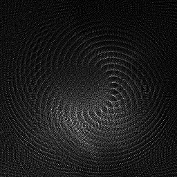
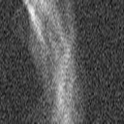
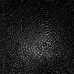
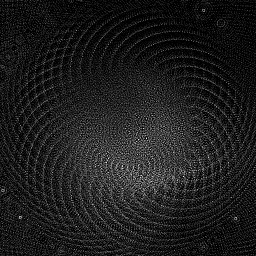
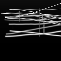
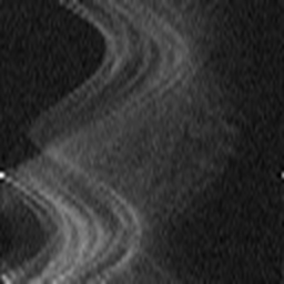
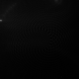
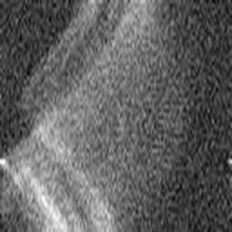
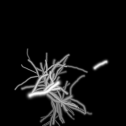
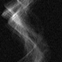
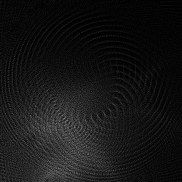
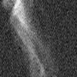
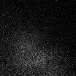
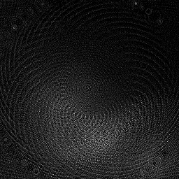
Reconstruction Gallery — 4 Scenes × 3 Scenarios
Method: CPU_baseline | Mismatch: nominal (nominal=True, perturbed=False)
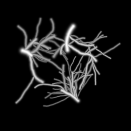
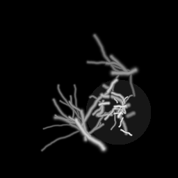
Ground Truth
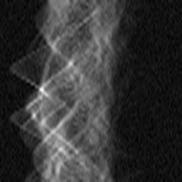
Measurement
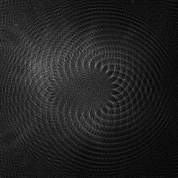
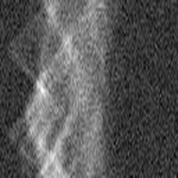
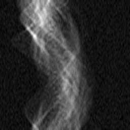
Reconstruction
Ground Truth
Measurement
Reconstruction
Ground Truth
Measurement (perturbed)
Reconstruction
Mean PSNR Across All Scenes
Per-scene PSNR breakdown (4 scenes)
| Scene | I (PSNR) | I (SSIM) | II (PSNR) | II (SSIM) | III (PSNR) | III (SSIM) |
|---|---|---|---|---|---|---|
| scene_00 | 14.042007760383013 | 0.008958793645003293 | 13.598463335451205 | 0.007060754825687232 | 13.088380465365967 | 0.007256907559667703 |
| scene_01 | 16.19315378500214 | 0.01314146181335565 | 16.07522538005379 | 0.012612947124721307 | 15.839492757083356 | 0.009980624748049654 |
| scene_02 | 12.091974958245297 | 0.3322325227011648 | 12.356456773236392 | 0.11701569613853909 | 12.322206276496306 | 0.14220485543340522 |
| scene_03 | 15.97128333287741 | 0.041535267737212986 | 15.587704031026135 | 0.0222863921560889 | 15.086497239299302 | 0.016744711424171124 |
| Mean | 14.574604959126965 | 0.09896701147418419 | 14.40446237994188 | 0.03974394756125913 | 14.084144184561232 | 0.04404677479132342 |
Experimental Setup
Key References
- Wang & Yao, 'Photoacoustic microscopy and computed tomography', Nature Methods 13, 627-638 (2016)
- Manwar et al., 'OADAT: Optoacoustic dataset', J. Biophotonics 2024
Canonical Datasets
- OADAT (optoacoustic benchmark)
- IPASC consensus datasets
Spec DAG — Forward Model Pipeline
P(acoustic) → Σ_t → D(g, η₂)
Mismatch Parameters
| Symbol | Parameter | Description | Nominal | Perturbed |
|---|---|---|---|---|
| Δc | sos | Speed-of-sound error (m/s) | 1540 | 1560 |
| ΔΦ | fluence | Fluence distribution error (%) | 0 | 10.0 |
| Δh | sensor_response | Sensor impulse response error (%) | 0 | 5.0 |
Credits System
Spec Primitives Reference (11 primitives)
Free-space or medium propagation kernel (Fresnel, Rayleigh-Sommerfeld).
Spatial or spatio-temporal amplitude modulation (coded aperture, SLM pattern).
Geometric projection operator (Radon transform, fan-beam, cone-beam).
Sampling in the Fourier / k-space domain (MRI, ptychography).
Shift-invariant convolution with a point-spread function (PSF).
Summation along a physical dimension (spectral, temporal, angular).
Sensor readout with gain g and noise model η (Gaussian, Poisson, mixed).
Patterned illumination (block, Hadamard, random) applied to the scene.
Spectral dispersion element (prism, grating) with shift α and aperture a.
Sample or gantry rotation (CT, electron tomography).
Spectral filter or monochromator selecting a wavelength band.