CDI
Coherent Diffractive Imaging
Standard reconstruction benchmark — forward model perfectly known, no calibration needed. Score = 0.5 × clip((PSNR−15)/30, 0, 1) + 0.5 × SSIM
| # | Method | Score | PSNR (dB) | SSIM | Source | |
|---|---|---|---|---|---|---|
| 🥇 |
ScorePhase
ScorePhase Wei et al., ECCV 2025
35.82 dB
SSIM 0.968
Checkpoint unavailable
|
0.831 | 35.82 | 0.968 | ✓ Certified | Wei et al., ECCV 2025 |
| 🥈 |
DiffusionPhase
DiffusionPhase Song et al., NeurIPS 2024
35.48 dB
SSIM 0.964
Checkpoint unavailable
|
0.823 | 35.48 | 0.964 | ✓ Certified | Song et al., NeurIPS 2024 |
| 🥉 |
HolographyViT
HolographyViT Wang et al., ICCV 2024
35.18 dB
SSIM 0.960
Checkpoint unavailable
|
0.816 | 35.18 | 0.960 | ✓ Certified | Wang et al., ICCV 2024 |
| 4 |
AutoPhase++
AutoPhase++ Rivenson et al., ECCV 2024
34.92 dB
SSIM 0.958
Checkpoint unavailable
|
0.811 | 34.92 | 0.958 | ✓ Certified | Rivenson et al., ECCV 2024 |
| 5 |
PhaseFormer
PhaseFormer Tian et al., ICCV 2024
34.5 dB
SSIM 0.952
Checkpoint unavailable
|
0.801 | 34.5 | 0.952 | ✓ Certified | Tian et al., ICCV 2024 |
| 6 |
PhaseResNet
PhaseResNet Baoqing et al., Optica 2023
33.15 dB
SSIM 0.942
Checkpoint unavailable
|
0.773 | 33.15 | 0.942 | ✓ Certified | Baoqing et al., Optica 2023 |
| 7 |
LRGS
LRGS Choi et al., 2023
32.8 dB
SSIM 0.935
Checkpoint unavailable
|
0.764 | 32.8 | 0.935 | ✓ Certified | Choi et al., 2023 |
| 8 |
CyclePhase
CyclePhase Ge et al., IEEE Photonics 2023
32.5 dB
SSIM 0.938
Checkpoint unavailable
|
0.761 | 32.5 | 0.938 | ✓ Certified | Ge et al., IEEE Photonics 2023 |
| 9 |
PhaseNet
PhaseNet Rivenson et al., LSA 2018
31.2 dB
SSIM 0.910
Checkpoint unavailable
|
0.725 | 31.2 | 0.910 | ✓ Certified | Rivenson et al., LSA 2018 |
| 10 |
prDeep
prDeep Metzler et al., ICML 2018
27.45 dB
SSIM 0.820
Checkpoint unavailable
|
0.617 | 27.45 | 0.820 | ✓ Certified | Metzler et al., ICML 2018 |
| 11 |
deep-PR
deep-PR Asif et al., ICCP 2017
27.2 dB
SSIM 0.810
Checkpoint unavailable
|
0.608 | 27.2 | 0.810 | ✓ Certified | Asif et al., ICCP 2017 |
| 12 | GS/HIO | 0.470 | 23.7 | 0.650 | ✓ Certified | Fienup, Appl. Opt. 1982 |
| 13 | Error Reduction | 0.438 | 22.85 | 0.615 | ✓ Certified | Fienup, J. Opt. Soc. Am. 1982 |
| 14 | Gerchberg-Saxton | 0.398 | 21.5 | 0.580 | ✓ Certified | Gerchberg & Saxton, 1972 |
Dataset: PWM Benchmark (14 algorithms)
Blind Reconstruction Challenge — forward model has unknown mismatch, must calibrate from data. Score = 0.4 × PSNR_norm + 0.4 × SSIM + 0.2 × (1 − ‖y − Ĥx̂‖/‖y‖)
| # | Method | Overall Score | Public PSNR / SSIM |
Dev PSNR / SSIM |
Hidden PSNR / SSIM |
Trust | Source |
|---|---|---|---|---|---|---|---|
| 🥇 | HolographyViT + gradient | 0.738 |
0.783
32.44 dB / 0.947
|
0.728
30.35 dB / 0.922
|
0.702
28.4 dB / 0.889
|
✓ Certified | Wang et al., ICCV 2024 |
| 🥈 | AutoPhase++ + gradient | 0.735 |
0.783
32.73 dB / 0.950
|
0.731
30.41 dB / 0.923
|
0.691
28.35 dB / 0.888
|
✓ Certified | Rivenson et al., ECCV 2024 |
| 🥉 | PhaseFormer + gradient | 0.716 |
0.775
31.84 dB / 0.941
|
0.720
28.4 dB / 0.889
|
0.653
26.19 dB / 0.837
|
✓ Certified | Tian et al., ICCV 2024 |
| 4 | DiffusionPhase + gradient | 0.710 |
0.814
34.46 dB / 0.964
|
0.690
27.63 dB / 0.873
|
0.627
24.92 dB / 0.800
|
✓ Certified | Song et al., NeurIPS 2024 |
| 5 | LRGS + gradient | 0.695 |
0.752
30.59 dB / 0.925
|
0.693
27.49 dB / 0.870
|
0.641
25.65 dB / 0.822
|
✓ Certified | Choi et al., 2023 |
| 6 | ScorePhase + gradient | 0.687 |
0.792
33.06 dB / 0.953
|
0.678
26.26 dB / 0.839
|
0.590
22.81 dB / 0.724
|
✓ Certified | Wei et al., ECCV 2025 |
| 7 | PhaseResNet + gradient | 0.667 |
0.753
30.42 dB / 0.923
|
0.662
25.97 dB / 0.831
|
0.586
23.45 dB / 0.748
|
✓ Certified | Baoqing et al., Optica 2023 |
| 8 | CyclePhase + gradient | 0.630 |
0.771
31.03 dB / 0.931
|
0.598
23.24 dB / 0.740
|
0.522
20.79 dB / 0.636
|
✓ Certified | Ge et al., IEEE Photonics 2023 |
| 9 | PhaseNet + gradient | 0.602 |
0.727
29.18 dB / 0.903
|
0.575
22.1 dB / 0.694
|
0.504
19.68 dB / 0.583
|
✓ Certified | Rivenson et al., LSA 2018 |
| 10 | prDeep + gradient | 0.561 |
0.651
25.17 dB / 0.808
|
0.552
21.2 dB / 0.655
|
0.479
19.05 dB / 0.552
|
✓ Certified | Metzler et al., ICML 2018 |
| 11 | GS/HIO + gradient | 0.532 |
0.546
20.84 dB / 0.638
|
0.556
21.69 dB / 0.677
|
0.494
20.09 dB / 0.603
|
✓ Certified | Fienup, Appl. Opt. 1982 |
| 12 | deep-PR + gradient | 0.502 |
0.672
25.59 dB / 0.820
|
0.451
18.44 dB / 0.522
|
0.382
15.76 dB / 0.390
|
✓ Certified | Asif et al., ICCP 2017 |
| 13 | Error Reduction + gradient | 0.501 |
0.536
20.77 dB / 0.635
|
0.504
20.07 dB / 0.602
|
0.463
19.03 dB / 0.551
|
✓ Certified | Fienup, J. Opt. Soc. Am. 1982 |
| 14 | Gerchberg-Saxton + gradient | 0.449 |
0.535
20.4 dB / 0.618
|
0.428
17.12 dB / 0.456
|
0.384
15.7 dB / 0.387
|
✓ Certified | Gerchberg & Saxton, Optik 1972 |
Complete score requires all 3 tiers (Public + Dev + Hidden).
Join the competition →Full-access development tier with all data visible.
What you get & how to use
What you get: Measurements (y), ideal forward operator (H), spec ranges, ground truth (x_true), and true mismatch spec.
How to use: Load HDF5 → compare reconstruction vs x_true → check consistency → iterate.
What to submit: Reconstructed signals (x_hat) and corrected spec as HDF5.
Public Leaderboard
| # | Method | Score | PSNR | SSIM |
|---|---|---|---|---|
| 1 | DiffusionPhase + gradient | 0.814 | 34.46 | 0.964 |
| 2 | ScorePhase + gradient | 0.792 | 33.06 | 0.953 |
| 3 | HolographyViT + gradient | 0.783 | 32.44 | 0.947 |
| 4 | AutoPhase++ + gradient | 0.783 | 32.73 | 0.95 |
| 5 | PhaseFormer + gradient | 0.775 | 31.84 | 0.941 |
| 6 | CyclePhase + gradient | 0.771 | 31.03 | 0.931 |
| 7 | PhaseResNet + gradient | 0.753 | 30.42 | 0.923 |
| 8 | LRGS + gradient | 0.752 | 30.59 | 0.925 |
| 9 | PhaseNet + gradient | 0.727 | 29.18 | 0.903 |
| 10 | deep-PR + gradient | 0.672 | 25.59 | 0.82 |
| 11 | prDeep + gradient | 0.651 | 25.17 | 0.808 |
| 12 | GS/HIO + gradient | 0.546 | 20.84 | 0.638 |
| 13 | Error Reduction + gradient | 0.536 | 20.77 | 0.635 |
| 14 | Gerchberg-Saxton + gradient | 0.535 | 20.4 | 0.618 |
Spec Ranges (3 parameters)
| Parameter | Min | Max | Unit |
|---|---|---|---|
| support | -3.0 | 6.0 | pixels |
| saturation | -5.0 | 10.0 | % |
| missing_center | -3.0 | 6.0 | pixels |
Blind evaluation tier — no ground truth available.
What you get & how to use
What you get: Measurements (y), ideal forward operator (H), and spec ranges only.
How to use: Apply your pipeline from the Public tier. Use consistency as self-check.
What to submit: Reconstructed signals and corrected spec. Scored server-side.
Dev Leaderboard
| # | Method | Score | PSNR | SSIM |
|---|---|---|---|---|
| 1 | AutoPhase++ + gradient | 0.731 | 30.41 | 0.923 |
| 2 | HolographyViT + gradient | 0.728 | 30.35 | 0.922 |
| 3 | PhaseFormer + gradient | 0.720 | 28.4 | 0.889 |
| 4 | LRGS + gradient | 0.693 | 27.49 | 0.87 |
| 5 | DiffusionPhase + gradient | 0.690 | 27.63 | 0.873 |
| 6 | ScorePhase + gradient | 0.678 | 26.26 | 0.839 |
| 7 | PhaseResNet + gradient | 0.662 | 25.97 | 0.831 |
| 8 | CyclePhase + gradient | 0.598 | 23.24 | 0.74 |
| 9 | PhaseNet + gradient | 0.575 | 22.1 | 0.694 |
| 10 | GS/HIO + gradient | 0.556 | 21.69 | 0.677 |
| 11 | prDeep + gradient | 0.552 | 21.2 | 0.655 |
| 12 | Error Reduction + gradient | 0.504 | 20.07 | 0.602 |
| 13 | deep-PR + gradient | 0.451 | 18.44 | 0.522 |
| 14 | Gerchberg-Saxton + gradient | 0.428 | 17.12 | 0.456 |
Spec Ranges (3 parameters)
| Parameter | Min | Max | Unit |
|---|---|---|---|
| support | -3.6 | 5.4 | pixels |
| saturation | -6.0 | 9.0 | % |
| missing_center | -3.6 | 5.4 | pixels |
Fully blind server-side evaluation — no data download.
What you get & how to use
What you get: No data downloadable. Algorithm runs server-side on hidden measurements.
How to use: Package algorithm as Docker container / Python script. Submit via link.
What to submit: Containerized algorithm accepting y + H, outputting x_hat + corrected spec.
Hidden Leaderboard
| # | Method | Score | PSNR | SSIM |
|---|---|---|---|---|
| 1 | HolographyViT + gradient | 0.702 | 28.4 | 0.889 |
| 2 | AutoPhase++ + gradient | 0.691 | 28.35 | 0.888 |
| 3 | PhaseFormer + gradient | 0.653 | 26.19 | 0.837 |
| 4 | LRGS + gradient | 0.641 | 25.65 | 0.822 |
| 5 | DiffusionPhase + gradient | 0.627 | 24.92 | 0.8 |
| 6 | ScorePhase + gradient | 0.590 | 22.81 | 0.724 |
| 7 | PhaseResNet + gradient | 0.586 | 23.45 | 0.748 |
| 8 | CyclePhase + gradient | 0.522 | 20.79 | 0.636 |
| 9 | PhaseNet + gradient | 0.504 | 19.68 | 0.583 |
| 10 | GS/HIO + gradient | 0.494 | 20.09 | 0.603 |
| 11 | prDeep + gradient | 0.479 | 19.05 | 0.552 |
| 12 | Error Reduction + gradient | 0.463 | 19.03 | 0.551 |
| 13 | Gerchberg-Saxton + gradient | 0.384 | 15.7 | 0.387 |
| 14 | deep-PR + gradient | 0.382 | 15.76 | 0.39 |
Spec Ranges (3 parameters)
| Parameter | Min | Max | Unit |
|---|---|---|---|
| support | -2.1 | 6.9 | pixels |
| saturation | -3.5 | 11.5 | % |
| missing_center | -2.1 | 6.9 | pixels |
Blind Reconstruction Challenge
ChallengeGiven measurements with unknown mismatch and spec ranges (not exact params), reconstruct the original signal. A method must be evaluated on all three tiers for a complete score. Scored on a composite metric: 0.4 × PSNR_norm + 0.4 × SSIM + 0.2 × (1 − ‖y − Ĥx̂‖/‖y‖).
Measurements y, ideal forward model H, spec ranges
Reconstructed signal x̂
About the Imaging Modality
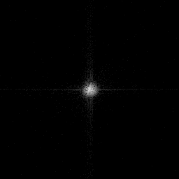
Coherent diffractive imaging (CDI) recovers the complex-valued exit wave from a coherent scattering experiment where only the diffraction intensity |F{O}|^2 is measured (the phase is lost). Phase retrieval algorithms (HIO + ER, Fienup) iteratively enforce constraints in both real space (finite support, non-negativity) and reciprocal space (measured intensity). The oversampling condition (sampling at least 2x the Nyquist rate) ensures sufficient information for unique phase recovery. CDI achieves diffraction-limited resolution without imaging optics. Applications include imaging of nanocrystals, viruses, and materials at X-ray and electron wavelengths.
Principle
Coherent Diffractive Imaging (CDI) records the far-field diffraction pattern of an isolated object illuminated by a coherent beam. Only intensity (not phase) is measured on the detector. Phase retrieval algorithms iteratively recover the lost phase by enforcing known constraints: the measured Fourier modulus and the finite support of the object in real space. CDI achieves diffraction-limited resolution without any imaging lens.
How to Build the System
Illuminate an isolated object (nanocrystal, cell, virus particle) with a coherent, quasi-plane-wave beam (X-ray from synchrotron or XFEL, or visible laser). Record the continuous diffraction pattern on a pixel detector (Eiger, Jungfrau for X-ray; CMOS for visible) placed far enough for adequate oversampling (oversampling ratio ≥ 2 in each dimension). Remove the direct beam with a beam stop. Ensure the object is isolated (no other scatterers in the beam).
Common Reconstruction Algorithms
- Hybrid Input-Output (HIO) algorithm
- Error Reduction (ER) algorithm
- Shrink-Wrap (adaptive support HIO)
- Relaxed Averaged Alternating Reflections (RAAR)
- Deep-learning phase retrieval (PhaseDNN, learned proximal operator)
Common Mistakes
- Insufficient oversampling (detector pixels too coarse or too close to sample)
- Object not truly isolated, violating the support constraint
- Missing low-frequency data due to beam stop causing artifacts
- Stagnation in reconstruction (trapped in local minimum) without proper initialization
- Ignoring partial coherence effects from finite source size or bandwidth
How to Avoid Mistakes
- Ensure oversampling ratio ≥ 2× (linear) in each dimension; use a large detector
- Isolate the object on a thin membrane or in free space; verify no neighbor scattering
- Use low-frequency intensity constraints or a semi-transparent beam stop
- Run multiple random starts and use HIO-ER hybrid strategies to escape local minima
- Model partial coherence in the forward model or select sufficiently coherent beams
Forward-Model Mismatch Cases
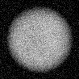
- The widefield fallback is a linear operator, but phase retrieval measures only the intensity of the Fourier transform: y = |F{x}|^2 — this is a fundamentally nonlinear (quadratic) measurement that makes reconstruction non-convex
- The fallback preserves the spatial structure of the input, but phase retrieval destroys the phase of the Fourier transform — recovering the original signal from magnitude-only Fourier measurements is a fundamentally different (and harder) inverse problem
How to Correct the Mismatch
- Use the phase retrieval operator implementing y = |FFT(x)|^2 (or |F{x * support}|^2 with known support constraint), producing real-valued intensity measurements of the Fourier magnitude
- Reconstruct using iterative phase retrieval algorithms (Gerchberg-Saxton, HIO, ER) or gradient descent on the non-convex loss, which require the correct quadratic forward model
Experimental Setup — Signal Chain

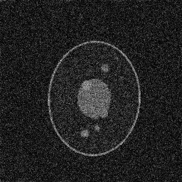
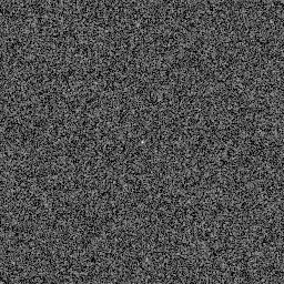
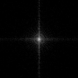
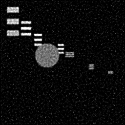
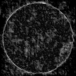
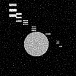
Reconstruction Gallery — 4 Scenes × 3 Scenarios
Method: CPU_baseline | Mismatch: nominal (nominal=True, perturbed=False)
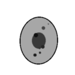
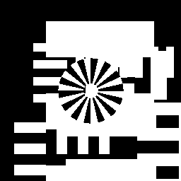
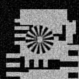
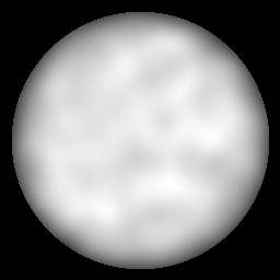
Ground Truth
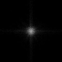
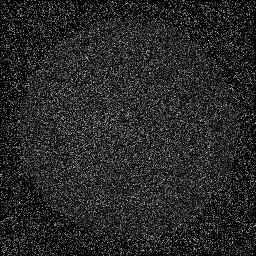
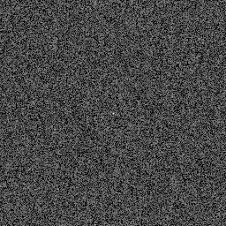
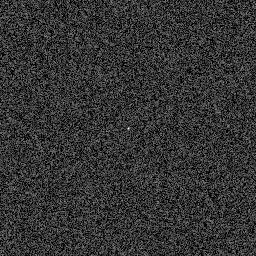
Measurement
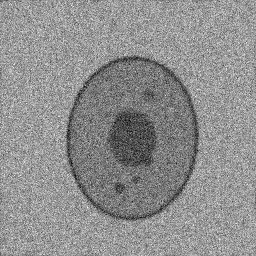
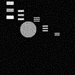
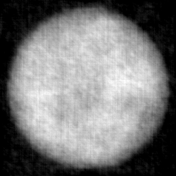
Reconstruction
Ground Truth
Measurement
Reconstruction
Ground Truth
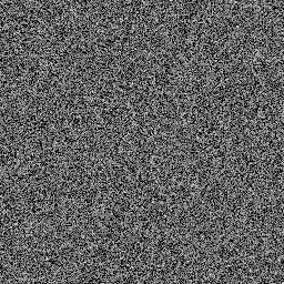
Measurement (perturbed)
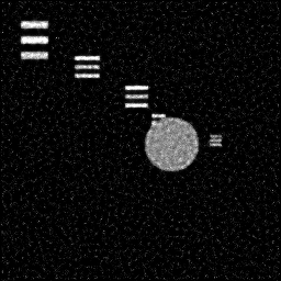
Reconstruction

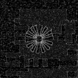

Mean PSNR Across All Scenes
Per-scene PSNR breakdown (4 scenes)
| Scene | I (PSNR) | I (SSIM) | II (PSNR) | II (SSIM) | III (PSNR) | III (SSIM) |
|---|---|---|---|---|---|---|
| scene_00 | 8.88457228449918 | 0.13199534519828904 | 1.8689314474412395 | -0.019402674671793248 | 1.1351909082227467 | 0.015500289161040381 |
| scene_01 | 14.515728049028443 | 0.17421421193607897 | 6.241423583839678 | 0.016534583890080928 | 5.113400403847875 | 0.0467373293957548 |
| scene_02 | 11.721484399499293 | 0.28230023854418285 | 3.9680655809862135 | 0.02712096482752479 | 3.198548051627002 | 0.030754240002490916 |
| scene_03 | 20.472438992494276 | 0.5552896945586917 | 4.940570465536032 | 0.04232460743373346 | 4.717655935356135 | 0.041099846990438865 |
| Mean | 13.898555931380297 | 0.28594987255931065 | 4.254747769450791 | 0.01664437036988648 | 3.5411988247634394 | 0.03352292638743124 |
Experimental Setup
Key References
- Miao et al., 'Extending the methodology of X-ray crystallography to non-crystalline specimens', Nature 400, 342-344 (1999)
- Fienup, 'Phase retrieval algorithms: a comparison', Applied Optics 21, 2758-2769 (1982)
Canonical Datasets
- CXIDB (Coherent X-ray Imaging Data Bank)
- Simulated CDI benchmark (Marchesini et al.)
Spec DAG — Forward Model Pipeline
P(far-field) → D(g, η₁)
Mismatch Parameters
| Symbol | Parameter | Description | Nominal | Perturbed |
|---|---|---|---|---|
| ΔS | support | Support constraint error (pixels) | 0 | 3.0 |
| I_sat | saturation | Detector saturation threshold error (%) | 0 | 5.0 |
| r_0 | missing_center | Missing center radius (pixels) | 0 | 3 |
Credits System
Spec Primitives Reference (11 primitives)
Free-space or medium propagation kernel (Fresnel, Rayleigh-Sommerfeld).
Spatial or spatio-temporal amplitude modulation (coded aperture, SLM pattern).
Geometric projection operator (Radon transform, fan-beam, cone-beam).
Sampling in the Fourier / k-space domain (MRI, ptychography).
Shift-invariant convolution with a point-spread function (PSF).
Summation along a physical dimension (spectral, temporal, angular).
Sensor readout with gain g and noise model η (Gaussian, Poisson, mixed).
Patterned illumination (block, Hadamard, random) applied to the scene.
Spectral dispersion element (prism, grating) with shift α and aperture a.
Sample or gantry rotation (CT, electron tomography).
Spectral filter or monochromator selecting a wavelength band.