Panorama
Panorama Multi-Focus Fusion
Standard reconstruction benchmark — forward model perfectly known, no calibration needed. Score = 0.5 × clip((PSNR−15)/30, 0, 1) + 0.5 × SSIM
| # | Method | Score | PSNR (dB) | SSIM | Source | |
|---|---|---|---|---|---|---|
| 🥇 |
PanoFormer
PanoFormer Image stitching transformer, 2024
35.0 dB
SSIM 0.950
Checkpoint unavailable
|
0.808 | 35.0 | 0.950 | ✓ Certified | Image stitching transformer, 2024 |
| 🥈 |
UDIS
UDIS Nie et al., ICCV 2021
33.0 dB
SSIM 0.920
Checkpoint unavailable
|
0.760 | 33.0 | 0.920 | ✓ Certified | Nie et al., ICCV 2021 |
| 🥉 | APAP | 0.667 | 29.5 | 0.850 | ✓ Certified | Zaragoza et al., CVPR 2013 |
| 4 | SIFT-RANSAC | 0.553 | 26.0 | 0.740 | ✓ Certified | Lowe, IJCV 2004 |
Dataset: PWM Benchmark (4 algorithms)
Blind Reconstruction Challenge — forward model has unknown mismatch, must calibrate from data. Score = 0.4 × PSNR_norm + 0.4 × SSIM + 0.2 × (1 − ‖y − Ĥx̂‖/‖y‖)
| # | Method | Overall Score | Public PSNR / SSIM |
Dev PSNR / SSIM |
Hidden PSNR / SSIM |
Trust | Source |
|---|---|---|---|---|---|---|---|
| 🥇 | PanoFormer + gradient | 0.727 |
0.784
32.79 dB / 0.951
|
0.726
29.83 dB / 0.914
|
0.671
26.89 dB / 0.855
|
✓ Certified | Image stitching transformer, 2024 |
| 🥈 | UDIS + gradient | 0.666 |
0.755
30.81 dB / 0.928
|
0.649
25.01 dB / 0.803
|
0.594
23.86 dB / 0.764
|
✓ Certified | Nie et al., ICCV 2021 |
| 🥉 | APAP + gradient | 0.656 |
0.699
27.71 dB / 0.875
|
0.655
25.26 dB / 0.810
|
0.614
23.71 dB / 0.758
|
✓ Certified | Zaragoza et al., CVPR 2013 |
| 4 | SIFT-RANSAC + gradient | 0.593 |
0.625
24.21 dB / 0.776
|
0.599
23.01 dB / 0.731
|
0.556
21.76 dB / 0.680
|
✓ Certified | Lowe, IJCV 2004 |
Complete score requires all 3 tiers (Public + Dev + Hidden).
Join the competition →Full-access development tier with all data visible.
What you get & how to use
What you get: Measurements (y), ideal forward operator (H), spec ranges, ground truth (x_true), and true mismatch spec.
How to use: Load HDF5 → compare reconstruction vs x_true → check consistency → iterate.
What to submit: Reconstructed signals (x_hat) and corrected spec as HDF5.
Public Leaderboard
| # | Method | Score | PSNR | SSIM |
|---|---|---|---|---|
| 1 | PanoFormer + gradient | 0.784 | 32.79 | 0.951 |
| 2 | UDIS + gradient | 0.755 | 30.81 | 0.928 |
| 3 | APAP + gradient | 0.699 | 27.71 | 0.875 |
| 4 | SIFT-RANSAC + gradient | 0.625 | 24.21 | 0.776 |
Spec Ranges (3 parameters)
| Parameter | Min | Max | Unit |
|---|---|---|---|
| focus_step | -2.0 | 4.0 | μm |
| registration | -0.5 | 1.0 | pixels |
| exposure_variation | -3.0 | 6.0 | % |
Blind evaluation tier — no ground truth available.
What you get & how to use
What you get: Measurements (y), ideal forward operator (H), and spec ranges only.
How to use: Apply your pipeline from the Public tier. Use consistency as self-check.
What to submit: Reconstructed signals and corrected spec. Scored server-side.
Dev Leaderboard
| # | Method | Score | PSNR | SSIM |
|---|---|---|---|---|
| 1 | PanoFormer + gradient | 0.726 | 29.83 | 0.914 |
| 2 | APAP + gradient | 0.655 | 25.26 | 0.81 |
| 3 | UDIS + gradient | 0.649 | 25.01 | 0.803 |
| 4 | SIFT-RANSAC + gradient | 0.599 | 23.01 | 0.731 |
Spec Ranges (3 parameters)
| Parameter | Min | Max | Unit |
|---|---|---|---|
| focus_step | -2.4 | 3.6 | μm |
| registration | -0.6 | 0.9 | pixels |
| exposure_variation | -3.6 | 5.4 | % |
Fully blind server-side evaluation — no data download.
What you get & how to use
What you get: No data downloadable. Algorithm runs server-side on hidden measurements.
How to use: Package algorithm as Docker container / Python script. Submit via link.
What to submit: Containerized algorithm accepting y + H, outputting x_hat + corrected spec.
Hidden Leaderboard
| # | Method | Score | PSNR | SSIM |
|---|---|---|---|---|
| 1 | PanoFormer + gradient | 0.671 | 26.89 | 0.855 |
| 2 | APAP + gradient | 0.614 | 23.71 | 0.758 |
| 3 | UDIS + gradient | 0.594 | 23.86 | 0.764 |
| 4 | SIFT-RANSAC + gradient | 0.556 | 21.76 | 0.68 |
Spec Ranges (3 parameters)
| Parameter | Min | Max | Unit |
|---|---|---|---|
| focus_step | -1.4 | 4.6 | μm |
| registration | -0.35 | 1.15 | pixels |
| exposure_variation | -2.1 | 6.9 | % |
Blind Reconstruction Challenge
ChallengeGiven measurements with unknown mismatch and spec ranges (not exact params), reconstruct the original signal. A method must be evaluated on all three tiers for a complete score. Scored on a composite metric: 0.4 × PSNR_norm + 0.4 × SSIM + 0.2 × (1 − ‖y − Ĥx̂‖/‖y‖).
Measurements y, ideal forward model H, spec ranges
Reconstructed signal x̂
About the Imaging Modality
Multi-focus panoramic fusion combines images captured at different focal planes and/or different spatial positions to produce an all-in-focus image with extended depth of field and wide field of view. Focus stacking selects the sharpest regions from each focal plane using local contrast measures, then blends them via Laplacian pyramid fusion or wavelet-based methods. Panoramic stitching aligns overlapping images using feature matching (SIFT/SURF) and blends seams. Primary challenges include parallax at scene edges and focus measure ambiguity in low-texture regions.
Principle
Panoramic multi-focus fusion captures multiple images of the same wide scene at different focal distances and combines them to produce a single all-in-focus panorama with extended depth of field. Image stitching aligns overlapping frames using feature matching and homography estimation, while focus fusion selects the sharpest pixels from each focal plane.
How to Build the System
Mount a camera on a motorized panoramic head (nodal point rotation). For each pan/tilt position, capture a focus stack (3-10 images at different focus distances). Use a medium-aperture setting (f/5.6-f/8) for each frame. Stitch overlapping views (30 % horizontal overlap) and fuse focus stacks per view tile. Calibrate the panoramic head to rotate around the lens entrance pupil to minimize parallax.
Common Reconstruction Algorithms
- Laplacian pyramid focus fusion (weighted blending by local contrast)
- SIFT/SURF feature matching + RANSAC homography estimation
- Multi-band blending (Burt-Adelson) for seamless stitching
- Exposure fusion (Mertens et al.) for HDR panoramas
- Deep-learning focus stacking (DFDF, DeepFocus)
Common Mistakes
- Parallax errors from rotation not centered on the lens entrance pupil
- Ghosting from moving objects between sequential captures
- Color inconsistency between overlapping tiles due to auto-exposure variation
- Incomplete focus coverage leaving blurry regions in the final panorama
- Stitching artifacts at seam lines visible in the final output
How to Avoid Mistakes
- Use a calibrated panoramic head; verify no-parallax point for the specific lens
- Mask out or blend moving objects; capture quickly or use simultaneous multi-camera rigs
- Lock exposure, white balance, and focus (manual mode) across all tiles
- Plan focus distances to cover the entire depth range of the scene
- Use multi-band blending and choose seam lines in textureless regions
Forward-Model Mismatch Cases
- The widefield fallback applies Gaussian blur to a single image, but panoramic imaging involves geometric projection (cylindrical, spherical, or equirectangular) of the scene onto a wide field of view — the projection geometry is absent
- Panorama multi-focus fusion requires modeling focus variation across the wide FOV and stitching multiple exposures — the widefield single-frame model cannot capture the spatially varying focus or overlap regions
How to Correct the Mismatch
- Use the panorama operator that models the geometric projection (cylindrical or spherical warping) and focus-dependent blur across the wide field of view
- Reconstruct using image stitching with homography estimation, exposure fusion, and spatially varying deblurring that account for the correct projection geometry
Experimental Setup — Signal Chain

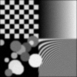
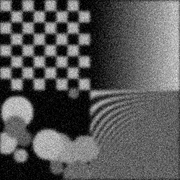
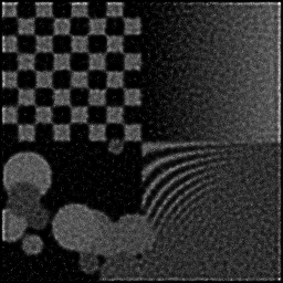
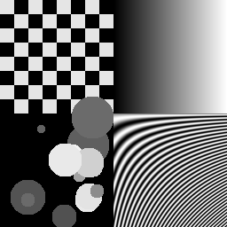
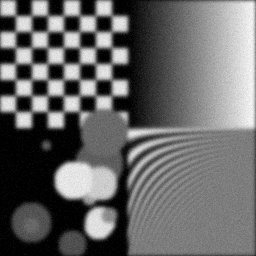
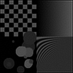
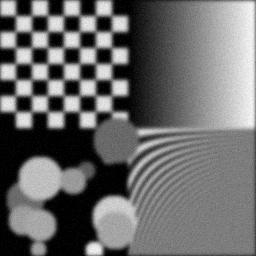
Reconstruction Gallery — 4 Scenes × 3 Scenarios
Method: CPU_baseline | Mismatch: nominal (nominal=True, perturbed=False)

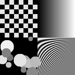
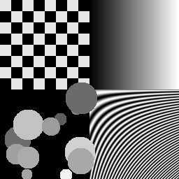
Ground Truth
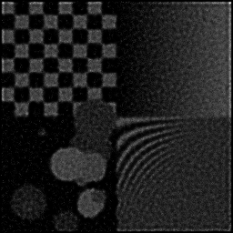
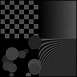
Measurement

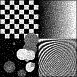
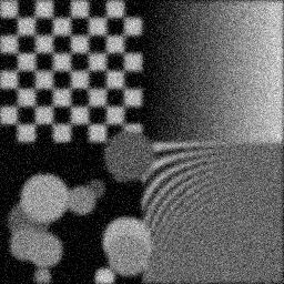
Reconstruction
Ground Truth
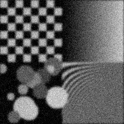
Measurement
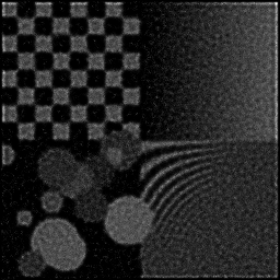
Reconstruction
Ground Truth
Measurement (perturbed)

Reconstruction


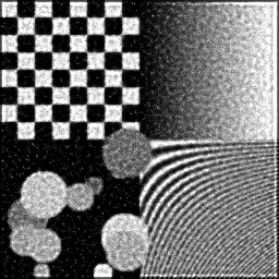
Mean PSNR Across All Scenes
Per-scene PSNR breakdown (4 scenes)
| Scene | I (PSNR) | I (SSIM) | II (PSNR) | II (SSIM) | III (PSNR) | III (SSIM) |
|---|---|---|---|---|---|---|
| scene_00 | 7.571173064124359 | 0.3615423650336687 | 7.4787043554532 | 0.19183056162517473 | 15.877011561792095 | 0.43371088310804984 |
| scene_01 | 7.696275051470366 | 0.38332215792026303 | 7.84628185762466 | 0.19830484931809553 | 15.892411144666065 | 0.4210479658349237 |
| scene_02 | 7.974649369166899 | 0.3846392902527589 | 7.451966505304711 | 0.1929426619644849 | 16.022129586295627 | 0.41754865353673254 |
| scene_03 | 7.8395670635647985 | 0.3793851129719163 | 7.6728272486833315 | 0.19311764475591156 | 15.93892392838001 | 0.4166048155455938 |
| Mean | 7.770416137081606 | 0.37722223154465173 | 7.612444991766475 | 0.19404892941591667 | 15.93261905528345 | 0.422228079506325 |
Experimental Setup
Key References
- Burt & Adelson, 'The Laplacian Pyramid as a Compact Image Code', IEEE Trans. Commun. 31, 532-540 (1983)
Canonical Datasets
- Lytro multi-focus test set
Spec DAG — Forward Model Pipeline
C(PSF_focus) → Σ_f → D(g, η₁)
Mismatch Parameters
| Symbol | Parameter | Description | Nominal | Perturbed |
|---|---|---|---|---|
| Δf | focus_step | Focus step error (μm) | 0 | 2.0 |
| Δr | registration | Inter-frame registration error (pixels) | 0 | 0.5 |
| ΔE | exposure_variation | Exposure variation (%) | 0 | 3.0 |
Credits System
Spec Primitives Reference (11 primitives)
Free-space or medium propagation kernel (Fresnel, Rayleigh-Sommerfeld).
Spatial or spatio-temporal amplitude modulation (coded aperture, SLM pattern).
Geometric projection operator (Radon transform, fan-beam, cone-beam).
Sampling in the Fourier / k-space domain (MRI, ptychography).
Shift-invariant convolution with a point-spread function (PSF).
Summation along a physical dimension (spectral, temporal, angular).
Sensor readout with gain g and noise model η (Gaussian, Poisson, mixed).
Patterned illumination (block, Hadamard, random) applied to the scene.
Spectral dispersion element (prism, grating) with shift α and aperture a.
Sample or gantry rotation (CT, electron tomography).
Spectral filter or monochromator selecting a wavelength band.