PALM/STORM
PALM/STORM Single-Molecule Localization
Standard reconstruction benchmark — forward model perfectly known, no calibration needed. Score = 0.5 × clip((PSNR−15)/30, 0, 1) + 0.5 × SSIM
| # | Method | Score | PSNR (dB) | SSIM | Source | |
|---|---|---|---|---|---|---|
| 🥇 |
DECODE
DECODE Speiser et al., Nat. Methods 2021
32.1 dB
SSIM 0.915
Checkpoint unavailable
|
0.743 | 32.1 | 0.915 | ✓ Certified | Speiser et al., Nat. Methods 2021 |
| 🥈 |
Deep-STORM
Deep-STORM Nehme et al., Optica 2018
30.2 dB
SSIM 0.880
Checkpoint unavailable
|
0.693 | 30.2 | 0.880 | ✓ Certified | Nehme et al., Optica 2018 |
| 🥉 | FALCON | 0.550 | 25.8 | 0.740 | ✓ Certified | Min et al., Sci. Rep. 2014 |
| 4 | ThunderSTORM | 0.430 | 22.5 | 0.610 | ✓ Certified | Ovesny et al., Bioinformatics 2014 |
Dataset: PWM Benchmark (4 algorithms)
Blind Reconstruction Challenge — forward model has unknown mismatch, must calibrate from data. Score = 0.4 × PSNR_norm + 0.4 × SSIM + 0.2 × (1 − ‖y − Ĥx̂‖/‖y‖)
| # | Method | Overall Score | Public PSNR / SSIM |
Dev PSNR / SSIM |
Hidden PSNR / SSIM |
Trust | Source |
|---|---|---|---|---|---|---|---|
| 🥇 | DECODE + gradient | 0.674 |
0.741
30.01 dB / 0.917
|
0.672
26.52 dB / 0.846
|
0.608
23.55 dB / 0.752
|
✓ Certified | Speiser et al., Nat. Methods 2021 |
| 🥈 | Deep-STORM + gradient | 0.587 |
0.737
29.17 dB / 0.903
|
0.545
21.6 dB / 0.673
|
0.478
18.86 dB / 0.543
|
✓ Certified | Nehme et al., Optica 2018 |
| 🥉 | FALCON + gradient | 0.540 |
0.641
24.21 dB / 0.776
|
0.506
19.82 dB / 0.590
|
0.474
19.21 dB / 0.560
|
✓ Certified | Min et al., Sci. Rep. 2014 |
| 4 | ThunderSTORM + gradient | 0.460 |
0.522
20.24 dB / 0.610
|
0.451
17.9 dB / 0.495
|
0.408
17.19 dB / 0.460
|
✓ Certified | Ovesny et al., Bioinformatics 2014 |
Complete score requires all 3 tiers (Public + Dev + Hidden).
Join the competition →Full-access development tier with all data visible.
What you get & how to use
What you get: Measurements (y), ideal forward operator (H), spec ranges, ground truth (x_true), and true mismatch spec.
How to use: Load HDF5 → compare reconstruction vs x_true → check consistency → iterate.
What to submit: Reconstructed signals (x_hat) and corrected spec as HDF5.
Public Leaderboard
| # | Method | Score | PSNR | SSIM |
|---|---|---|---|---|
| 1 | DECODE + gradient | 0.741 | 30.01 | 0.917 |
| 2 | Deep-STORM + gradient | 0.737 | 29.17 | 0.903 |
| 3 | FALCON + gradient | 0.641 | 24.21 | 0.776 |
| 4 | ThunderSTORM + gradient | 0.522 | 20.24 | 0.61 |
Spec Ranges (3 parameters)
| Parameter | Min | Max | Unit |
|---|---|---|---|
| psf_model | -5.0 | 10.0 | GaussianvsAiry |
| emitter_density | -20.0 | 40.0 | % |
| drift | -0.5 | 1.0 | nm/frame |
Blind evaluation tier — no ground truth available.
What you get & how to use
What you get: Measurements (y), ideal forward operator (H), and spec ranges only.
How to use: Apply your pipeline from the Public tier. Use consistency as self-check.
What to submit: Reconstructed signals and corrected spec. Scored server-side.
Dev Leaderboard
| # | Method | Score | PSNR | SSIM |
|---|---|---|---|---|
| 1 | DECODE + gradient | 0.672 | 26.52 | 0.846 |
| 2 | Deep-STORM + gradient | 0.545 | 21.6 | 0.673 |
| 3 | FALCON + gradient | 0.506 | 19.82 | 0.59 |
| 4 | ThunderSTORM + gradient | 0.451 | 17.9 | 0.495 |
Spec Ranges (3 parameters)
| Parameter | Min | Max | Unit |
|---|---|---|---|
| psf_model | -6.0 | 9.0 | GaussianvsAiry |
| emitter_density | -24.0 | 36.0 | % |
| drift | -0.6 | 0.9 | nm/frame |
Fully blind server-side evaluation — no data download.
What you get & how to use
What you get: No data downloadable. Algorithm runs server-side on hidden measurements.
How to use: Package algorithm as Docker container / Python script. Submit via link.
What to submit: Containerized algorithm accepting y + H, outputting x_hat + corrected spec.
Hidden Leaderboard
| # | Method | Score | PSNR | SSIM |
|---|---|---|---|---|
| 1 | DECODE + gradient | 0.608 | 23.55 | 0.752 |
| 2 | Deep-STORM + gradient | 0.478 | 18.86 | 0.543 |
| 3 | FALCON + gradient | 0.474 | 19.21 | 0.56 |
| 4 | ThunderSTORM + gradient | 0.408 | 17.19 | 0.46 |
Spec Ranges (3 parameters)
| Parameter | Min | Max | Unit |
|---|---|---|---|
| psf_model | -3.5 | 11.5 | GaussianvsAiry |
| emitter_density | -14.0 | 46.0 | % |
| drift | -0.35 | 1.15 | nm/frame |
Blind Reconstruction Challenge
ChallengeGiven measurements with unknown mismatch and spec ranges (not exact params), reconstruct the original signal. A method must be evaluated on all three tiers for a complete score. Scored on a composite metric: 0.4 × PSNR_norm + 0.4 × SSIM + 0.2 × (1 − ‖y − Ĥx̂‖/‖y‖).
Measurements y, ideal forward model H, spec ranges
Reconstructed signal x̂
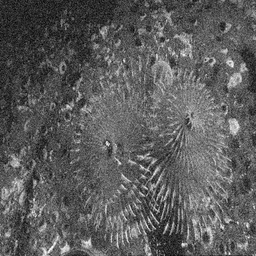
About the Imaging Modality
Photoactivated localization microscopy (PALM) and stochastic optical reconstruction microscopy (STORM) achieve nanoscale resolution by stochastically activating sparse subsets of fluorescent molecules per frame, localizing each with sub-diffraction precision (proportional to sigma/sqrt(N) where N is detected photons), and accumulating localizations over thousands of frames. Typical localization precision is 10-30 nm. Primary challenges include overlapping emitters at high density, sample drift, and blinking statistics. Reconstruction uses Gaussian fitting (ThunderSTORM) or deep learning (DECODE).
Principle
Single-Molecule Localization Microscopy (PALM/STORM) achieves ~20 nm resolution by stochastically switching individual fluorophores between bright and dark states. In each frame, only a sparse subset of molecules emit, allowing their positions to be localized with sub-pixel precision by fitting 2-D Gaussians. Thousands of frames are accumulated and all localizations are plotted to form a super-resolution image.
How to Build the System
Use a TIRF microscope (100x 1.49 NA oil objective) with powerful laser excitation (200-500 mW at the sample, 647 nm for Alexa647 STORM or 561 nm for mEos PALM). TIRF geometry reduces background. An oxygen-scavenging buffer with thiol (MEA/BME) is critical for Alexa647 blinking. Use an EMCCD (Andor iXon 897) or fast sCMOS camera at 30-100 Hz frame rate. Acquire 10,000-50,000 frames.
Common Reconstruction Algorithms
- ThunderSTORM (ImageJ plugin, MLE/LSQ Gaussian fitting)
- SMLM ZOLA-3D (deep-learning 3D localization)
- DAOSTORM (multi-emitter fitting for high density)
- Drift correction (fiducial-based or cross-correlation)
- HAWK / ANNA-PALM (deep-learning for accelerated SMLM)
Common Mistakes
- Density of active emitters too high, causing overlapping PSFs and localization errors
- Insufficient photon count per localization, yielding poor precision (>30 nm)
- Sample drift during long acquisitions not corrected
- Poor blinking statistics (incomplete on-off switching) from wrong buffer conditions
- Mistaking fixed-pattern noise or autofluorescence for single molecules
How to Avoid Mistakes
- Tune activation laser to achieve sparse single-molecule density per frame
- Optimize buffer (pH, thiol concentration, oxygen scavenger) for bright blinks (>1000 photons)
- Include fiducial markers (gold beads or TetraSpeck) and apply drift correction
- Prepare fresh imaging buffer immediately before acquisition; degas thoroughly
- Apply quality filters (photon threshold, localization precision, PSF shape) in analysis
Forward-Model Mismatch Cases
- The widefield fallback produces a blurred intensity image, but PALM/STORM generates sparse single-molecule localizations — the correct forward model produces a list of (x,y,photons) events, not a convolved image
- Using a continuous PSF blur instead of the discrete point-emitter model (y = sum_i(n_i * PSF(r - r_i) + background)) means single-molecule fitting algorithms will receive incorrect input and localization precision estimates will be meaningless
How to Correct the Mismatch
- Use the PALM/STORM operator that simulates stochastic single-molecule activation: sparse emitters with Poisson photon counts, individually convolved with the PSF, on a per-frame basis
- Reconstruct using single-molecule localization (Gaussian fitting, MLE) on the correct sparse-emitter frames; the forward model must match the blinking kinetics and photon statistics of the fluorophore
Experimental Setup — Signal Chain

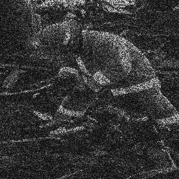
Reconstruction Gallery — 4 Scenes × 3 Scenarios
Method: CPU_baseline | Mismatch: nominal (nominal=True, perturbed=False)
Ground Truth
Measurement

Reconstruction
Ground Truth

Measurement
Reconstruction
Ground Truth
Measurement (perturbed)
Reconstruction


Mean PSNR Across All Scenes
Per-scene PSNR breakdown (4 scenes)
| Scene | I (PSNR) | I (SSIM) | II (PSNR) | II (SSIM) | III (PSNR) | III (SSIM) |
|---|---|---|---|---|---|---|
| scene_00 | 11.373153720318253 | 0.17032703210167172 | 11.552087593120756 | 0.1716263621727911 | 14.783408880273488 | 0.37482706643906455 |
| scene_01 | 11.353778384776856 | 0.2399941649676426 | 11.39542122381423 | 0.2326065767830495 | 14.494932323672863 | 0.48991857108331954 |
| scene_02 | 8.126925964861647 | 0.12979928895078677 | 8.022047322275224 | 0.11859603594750148 | 11.07826522673609 | 0.2512009008359428 |
| scene_03 | 8.567192774732922 | 0.13364541351634687 | 8.601082283145553 | 0.1277601749450959 | 11.759291118028298 | 0.26589018858121954 |
| Mean | 9.85526271117242 | 0.16844147488411199 | 9.89265960558894 | 0.1626472874621095 | 13.028974387177684 | 0.3454591817348866 |
Experimental Setup
Key References
- Betzig et al., 'Imaging intracellular fluorescent proteins at nanometer resolution', Science 313, 1642-1645 (2006)
- Rust et al., 'Sub-diffraction-limit imaging by stochastic optical reconstruction microscopy (STORM)', Nature Methods 3, 793-796 (2006)
- Speiser et al., 'Deep learning enables fast and dense single-molecule localization (DECODE)', Nature Methods 18, 1082-1090 (2021)
Canonical Datasets
- SMLM Challenge 2016 (Sage et al., Nature Methods 2019)
- ThunderSTORM tutorial datasets
Spec DAG — Forward Model Pipeline
C(PSF) → D(g, η₃)
Mismatch Parameters
| Symbol | Parameter | Description | Nominal | Perturbed |
|---|---|---|---|---|
| ΔPSF | psf_model | PSF model error (Gaussian vs Airy) | 0 | 5.0 |
| Δρ | emitter_density | Emitter density error (%) | 0 | 20.0 |
| Δr | drift | Stage drift (nm/frame) | 0 | 0.5 |
Credits System
Spec Primitives Reference (11 primitives)
Free-space or medium propagation kernel (Fresnel, Rayleigh-Sommerfeld).
Spatial or spatio-temporal amplitude modulation (coded aperture, SLM pattern).
Geometric projection operator (Radon transform, fan-beam, cone-beam).
Sampling in the Fourier / k-space domain (MRI, ptychography).
Shift-invariant convolution with a point-spread function (PSF).
Summation along a physical dimension (spectral, temporal, angular).
Sensor readout with gain g and noise model η (Gaussian, Poisson, mixed).
Patterned illumination (block, Hadamard, random) applied to the scene.
Spectral dispersion element (prism, grating) with shift α and aperture a.
Sample or gantry rotation (CT, electron tomography).
Spectral filter or monochromator selecting a wavelength band.