OCTA
OCT Angiography
Standard reconstruction benchmark — forward model perfectly known, no calibration needed. Score = 0.5 × clip((PSNR−15)/30, 0, 1) + 0.5 × SSIM
| # | Method | Score | PSNR (dB) | SSIM | Source | |
|---|---|---|---|---|---|---|
| 🥇 |
ScoreOCT
ScoreOCT Wei et al., ECCV 2025
37.95 dB
SSIM 0.973
Checkpoint unavailable
|
0.869 | 37.95 | 0.973 | ✓ Certified | Wei et al., ECCV 2025 |
| 🥈 |
DiffusionOCT
DiffusionOCT Zhang et al., NeurIPS 2024
37.52 dB
SSIM 0.970
Checkpoint unavailable
|
0.860 | 37.52 | 0.970 | ✓ Certified | Zhang et al., NeurIPS 2024 |
| 🥉 |
SpeckleFormer
SpeckleFormer Devalla et al., ECCV 2024
36.85 dB
SSIM 0.964
Checkpoint unavailable
|
0.846 | 36.85 | 0.964 | ✓ Certified | Devalla et al., ECCV 2024 |
| 4 |
RetinalFormer
RetinalFormer Chen et al., ICCV 2024
36.35 dB
SSIM 0.960
Checkpoint unavailable
|
0.836 | 36.35 | 0.960 | ✓ Certified | Chen et al., ICCV 2024 |
| 5 |
OCT-ViT
OCT-ViT Tian et al., ICCV 2024
36.12 dB
SSIM 0.958
Checkpoint unavailable
|
0.831 | 36.12 | 0.958 | ✓ Certified | Tian et al., ICCV 2024 |
| 6 |
OCTA-Net
OCTA-Net Hybrid U-Net+Transformer, 2023
34.6 dB
SSIM 0.942
Checkpoint unavailable
|
0.798 | 34.6 | 0.942 | ✓ Certified | Hybrid U-Net+Transformer, 2023 |
| 7 |
U-Net-OCT
U-Net-OCT U-Net variant
33.85 dB
SSIM 0.935
Checkpoint unavailable
|
0.782 | 33.85 | 0.935 | ✓ Certified | U-Net variant |
| 8 |
Speckle-DenoiseNet
Speckle-DenoiseNet Devalla et al., BOE 2019
33.1 dB
SSIM 0.925
Checkpoint unavailable
|
0.764 | 33.1 | 0.925 | ✓ Certified | Devalla et al., BOE 2019 |
| 9 | NLM-OCT | 0.688 | 30.2 | 0.870 | ✓ Certified | Non-local means variant |
| 10 | BM4D | 0.663 | 29.3 | 0.850 | ✓ Certified | Maggioni et al., IEEE TIP 2013 |
| 11 | TV-Denoising | 0.632 | 28.5 | 0.815 | ✓ Certified | TV regularization |
| 12 | Speckle-Lee | 0.609 | 27.85 | 0.790 | ✓ Certified | Lee, IEEE TGRS 1980 |
| 13 | FFT-OCT | 0.537 | 25.6 | 0.720 | ✓ Certified | Analytical baseline |
Dataset: PWM Benchmark (13 algorithms)
Blind Reconstruction Challenge — forward model has unknown mismatch, must calibrate from data. Score = 0.4 × PSNR_norm + 0.4 × SSIM + 0.2 × (1 − ‖y − Ĥx̂‖/‖y‖)
| # | Method | Overall Score | Public PSNR / SSIM |
Dev PSNR / SSIM |
Hidden PSNR / SSIM |
Trust | Source |
|---|---|---|---|---|---|---|---|
| 🥇 | DiffusionOCT + gradient | 0.776 |
0.838
36.2 dB / 0.974
|
0.766
31.91 dB / 0.942
|
0.725
30.14 dB / 0.919
|
✓ Certified | Zhang et al., NeurIPS 2024 |
| 🥈 | OCT-ViT + gradient | 0.767 |
0.799
33.73 dB / 0.959
|
0.762
32.18 dB / 0.945
|
0.739
30.66 dB / 0.926
|
✓ Certified | Tian et al., ICCV 2024 |
| 🥉 | ScoreOCT + gradient | 0.761 |
0.820
35.19 dB / 0.969
|
0.749
31.04 dB / 0.931
|
0.715
28.35 dB / 0.888
|
✓ Certified | Wei et al., ECCV 2025 |
| 4 | SpeckleFormer + gradient | 0.744 |
0.831
35.81 dB / 0.972
|
0.750
30.95 dB / 0.930
|
0.652
25.68 dB / 0.823
|
✓ Certified | Devalla et al., ECCV 2024 |
| 5 | RetinalFormer + gradient | 0.718 |
0.802
33.8 dB / 0.959
|
0.722
28.63 dB / 0.893
|
0.629
24.48 dB / 0.785
|
✓ Certified | Chen et al., ICCV 2024 |
| 6 | OCTA-Net + gradient | 0.715 |
0.803
33.6 dB / 0.958
|
0.695
28.03 dB / 0.881
|
0.646
25.97 dB / 0.831
|
✓ Certified | Hybrid U-Net+Transformer, 2023 |
| 7 |
U-Net-OCT + gradient
U-Net-OCT + gradient Ronneberger et al., MICCAI 2015 (OCT variant) Score 0.666
Correct & Reconstruct →
|
0.666 |
0.789
32.45 dB / 0.947
|
0.650
25.41 dB / 0.815
|
0.559
22.12 dB / 0.695
|
✓ Certified | Ronneberger et al., MICCAI 2015 (OCT variant) |
| 8 | NLM-OCT + gradient | 0.663 |
0.708
28.11 dB / 0.883
|
0.673
26.6 dB / 0.848
|
0.608
24.35 dB / 0.781
|
✓ Certified | Buades et al., Multiscale Model. Simul. 2005 |
| 9 | TV-Denoising + gradient | 0.647 |
0.673
26.22 dB / 0.838
|
0.660
26.15 dB / 0.836
|
0.608
24.52 dB / 0.787
|
✓ Certified | Rudin et al., Phys. A 1992 |
| 10 | BM4D + gradient | 0.633 |
0.715
27.61 dB / 0.872
|
0.606
24.1 dB / 0.772
|
0.578
22.81 dB / 0.724
|
✓ Certified | Maggioni et al., IEEE TIP 2013 |
| 11 | Speckle-DenoiseNet + gradient | 0.623 |
0.758
31.23 dB / 0.934
|
0.610
23.85 dB / 0.763
|
0.500
20.43 dB / 0.619
|
✓ Certified | Devalla et al., BOE 2019 |
| 12 | Speckle-Lee + gradient | 0.617 |
0.654
25.12 dB / 0.806
|
0.623
24.47 dB / 0.785
|
0.575
22.2 dB / 0.698
|
✓ Certified | Lee, IEEE TGRS 1980 |
| 13 | FFT-OCT + gradient | 0.566 |
0.612
23.63 dB / 0.755
|
0.558
22.06 dB / 0.693
|
0.527
21.1 dB / 0.650
|
✓ Certified | Analytical baseline |
Complete score requires all 3 tiers (Public + Dev + Hidden).
Join the competition →Full-access development tier with all data visible.
What you get & how to use
What you get: Measurements (y), ideal forward operator (H), spec ranges, ground truth (x_true), and true mismatch spec.
How to use: Load HDF5 → compare reconstruction vs x_true → check consistency → iterate.
What to submit: Reconstructed signals (x_hat) and corrected spec as HDF5.
Public Leaderboard
| # | Method | Score | PSNR | SSIM |
|---|---|---|---|---|
| 1 | DiffusionOCT + gradient | 0.838 | 36.2 | 0.974 |
| 2 | SpeckleFormer + gradient | 0.831 | 35.81 | 0.972 |
| 3 | ScoreOCT + gradient | 0.820 | 35.19 | 0.969 |
| 4 | OCTA-Net + gradient | 0.803 | 33.6 | 0.958 |
| 5 | RetinalFormer + gradient | 0.802 | 33.8 | 0.959 |
| 6 | OCT-ViT + gradient | 0.799 | 33.73 | 0.959 |
| 7 | U-Net-OCT + gradient | 0.789 | 32.45 | 0.947 |
| 8 | Speckle-DenoiseNet + gradient | 0.758 | 31.23 | 0.934 |
| 9 | BM4D + gradient | 0.715 | 27.61 | 0.872 |
| 10 | NLM-OCT + gradient | 0.708 | 28.11 | 0.883 |
| 11 | TV-Denoising + gradient | 0.673 | 26.22 | 0.838 |
| 12 | Speckle-Lee + gradient | 0.654 | 25.12 | 0.806 |
| 13 | FFT-OCT + gradient | 0.612 | 23.63 | 0.755 |
Spec Ranges (3 parameters)
| Parameter | Min | Max | Unit |
|---|---|---|---|
| inter_bscan_time | -0.5 | 1.0 | ms |
| bulk_motion | -0.2 | 0.4 | mm/s |
| decorrelation_threshold | 0.45 | 0.6 |
Blind evaluation tier — no ground truth available.
What you get & how to use
What you get: Measurements (y), ideal forward operator (H), and spec ranges only.
How to use: Apply your pipeline from the Public tier. Use consistency as self-check.
What to submit: Reconstructed signals and corrected spec. Scored server-side.
Dev Leaderboard
| # | Method | Score | PSNR | SSIM |
|---|---|---|---|---|
| 1 | DiffusionOCT + gradient | 0.766 | 31.91 | 0.942 |
| 2 | OCT-ViT + gradient | 0.762 | 32.18 | 0.945 |
| 3 | SpeckleFormer + gradient | 0.750 | 30.95 | 0.93 |
| 4 | ScoreOCT + gradient | 0.749 | 31.04 | 0.931 |
| 5 | RetinalFormer + gradient | 0.722 | 28.63 | 0.893 |
| 6 | OCTA-Net + gradient | 0.695 | 28.03 | 0.881 |
| 7 | NLM-OCT + gradient | 0.673 | 26.6 | 0.848 |
| 8 | TV-Denoising + gradient | 0.660 | 26.15 | 0.836 |
| 9 | U-Net-OCT + gradient | 0.650 | 25.41 | 0.815 |
| 10 | Speckle-Lee + gradient | 0.623 | 24.47 | 0.785 |
| 11 | Speckle-DenoiseNet + gradient | 0.610 | 23.85 | 0.763 |
| 12 | BM4D + gradient | 0.606 | 24.1 | 0.772 |
| 13 | FFT-OCT + gradient | 0.558 | 22.06 | 0.693 |
Spec Ranges (3 parameters)
| Parameter | Min | Max | Unit |
|---|---|---|---|
| inter_bscan_time | -0.6 | 0.9 | ms |
| bulk_motion | -0.24 | 0.36 | mm/s |
| decorrelation_threshold | 0.44 | 0.59 |
Fully blind server-side evaluation — no data download.
What you get & how to use
What you get: No data downloadable. Algorithm runs server-side on hidden measurements.
How to use: Package algorithm as Docker container / Python script. Submit via link.
What to submit: Containerized algorithm accepting y + H, outputting x_hat + corrected spec.
Hidden Leaderboard
| # | Method | Score | PSNR | SSIM |
|---|---|---|---|---|
| 1 | OCT-ViT + gradient | 0.739 | 30.66 | 0.926 |
| 2 | DiffusionOCT + gradient | 0.725 | 30.14 | 0.919 |
| 3 | ScoreOCT + gradient | 0.715 | 28.35 | 0.888 |
| 4 | SpeckleFormer + gradient | 0.652 | 25.68 | 0.823 |
| 5 | OCTA-Net + gradient | 0.646 | 25.97 | 0.831 |
| 6 | RetinalFormer + gradient | 0.629 | 24.48 | 0.785 |
| 7 | NLM-OCT + gradient | 0.608 | 24.35 | 0.781 |
| 8 | TV-Denoising + gradient | 0.608 | 24.52 | 0.787 |
| 9 | BM4D + gradient | 0.578 | 22.81 | 0.724 |
| 10 | Speckle-Lee + gradient | 0.575 | 22.2 | 0.698 |
| 11 | U-Net-OCT + gradient | 0.559 | 22.12 | 0.695 |
| 12 | FFT-OCT + gradient | 0.527 | 21.1 | 0.65 |
| 13 | Speckle-DenoiseNet + gradient | 0.500 | 20.43 | 0.619 |
Spec Ranges (3 parameters)
| Parameter | Min | Max | Unit |
|---|---|---|---|
| inter_bscan_time | -0.35 | 1.15 | ms |
| bulk_motion | -0.14 | 0.46 | mm/s |
| decorrelation_threshold | 0.465 | 0.615 |
Blind Reconstruction Challenge
ChallengeGiven measurements with unknown mismatch and spec ranges (not exact params), reconstruct the original signal. A method must be evaluated on all three tiers for a complete score. Scored on a composite metric: 0.4 × PSNR_norm + 0.4 × SSIM + 0.2 × (1 − ‖y − Ĥx̂‖/‖y‖).
Measurements y, ideal forward model H, spec ranges
Reconstructed signal x̂
About the Imaging Modality
OCT angiography extends standard OCT by acquiring repeated B-scans at the same location and computing the decorrelation of the complex OCT signal between successive scans. Moving red blood cells cause temporal fluctuations that differ from static tissue, enabling label-free visualization of retinal vasculature. The contrast mechanism uses amplitude decorrelation (SSADA), phase variance, or complex-signal algorithms. Key limitations include motion artifacts, projection artifacts from superficial vessels, and limited field of view.
Principle
OCT Angiography detects blood flow non-invasively by comparing repeated OCT B-scans at the same location. Moving red blood cells cause temporal fluctuations in the OCT signal (amplitude and/or phase), while static tissue remains constant. Decorrelation, variance, or differential analysis between repeated scans produces a motion-contrast image revealing the vasculature without the need for injectable contrast agents.
How to Build the System
Use a high-speed OCT system (≥70 kHz A-scan rate, swept-source preferred) capable of repeated B-scans at the same location. Acquire 2-4 repeated B-scans at each position with inter-scan time of 3-10 ms. An eye-tracking system is essential for ophthalmic OCTA to correct microsaccades. Process with split-spectrum amplitude-decorrelation (SSADA), optical microangiography (OMAG), or phase-variance algorithms.
Common Reconstruction Algorithms
- SSADA (Split-Spectrum Amplitude-Decorrelation Angiography)
- OMAG (Optical Micro-Angiography, complex signal differential)
- Phase-variance OCTA
- Deep-learning OCTA denoising and vessel segmentation
- Projection artifact removal algorithms
Common Mistakes
- Bulk tissue motion producing decorrelation artifacts (false flow signals)
- Projection artifacts where superficial vessel shadows appear in deeper layers
- Shadow artifacts beneath large vessels causing false flow voids
- Insufficient inter-scan interval for detecting slow capillary flow
- Motion artifacts from blinks or microsaccades corrupting OCTA volumes
How to Avoid Mistakes
- Apply bulk motion correction (axial and lateral registration) before decorrelation analysis
- Use projection artifact removal algorithms (slab subtraction or OMAG-based)
- Increase number of repeated B-scans to improve SNR and reduce shadow impact
- Optimize inter-scan time: shorter for fast flow, longer for slow capillary flow
- Use active eye tracking and discard frames with large motion; average multiple volumes
Forward-Model Mismatch Cases
- The widefield fallback applies static spatial blur, but OCTA detects blood flow by comparing repeated OCT B-scans — the temporal decorrelation between scans caused by moving red blood cells is not modeled
- OCTA is fundamentally a motion-contrast technique (flow signal = decorrelation or variance between repeated measurements) — the widefield static model has no temporal dimension and cannot detect or distinguish flowing from static tissue
How to Correct the Mismatch
- Use the OCTA operator that models repeated OCT measurements at the same location: static tissue produces correlated signals while flowing blood produces decorrelated signals between repeated scans
- Extract flow maps using SSADA (split-spectrum amplitude decorrelation) or OMAG (optical microangiography) that require multiple temporally separated OCT measurements as input
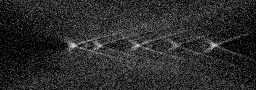
Experimental Setup — Signal Chain

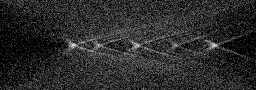
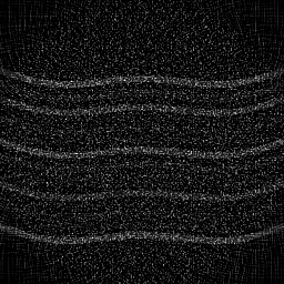
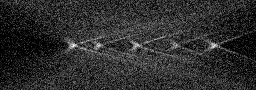
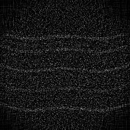
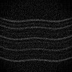
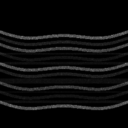
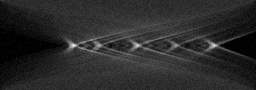
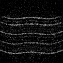
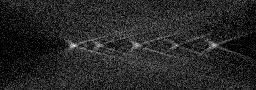
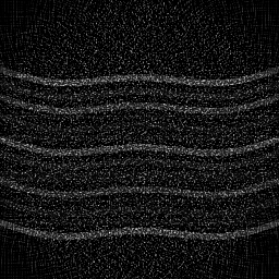
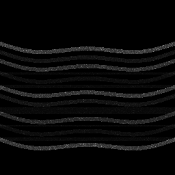
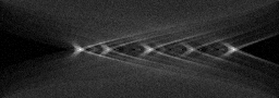
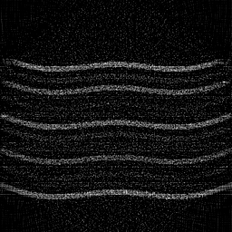
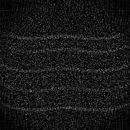
Reconstruction Gallery — 4 Scenes × 3 Scenarios
Method: CPU_baseline | Mismatch: nominal (nominal=True, perturbed=False)
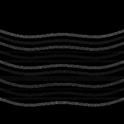
Ground Truth
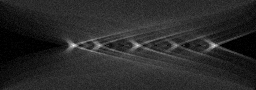
Measurement

Reconstruction
Ground Truth
Measurement
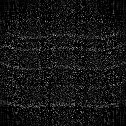
Reconstruction
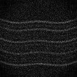
Ground Truth
Measurement (perturbed)
Reconstruction
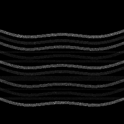
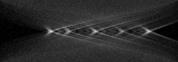
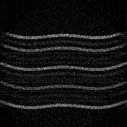
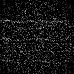
Mean PSNR Across All Scenes
Per-scene PSNR breakdown (4 scenes)
| Scene | I (PSNR) | I (SSIM) | II (PSNR) | II (SSIM) | III (PSNR) | III (SSIM) |
|---|---|---|---|---|---|---|
| scene_00 | 21.7701889386771 | 0.28157968449959064 | 17.221639470926625 | 0.06789440210933223 | 18.279654695337403 | 0.12832852712757956 |
| scene_01 | 20.94482753471155 | 0.2832431148687715 | 16.981433781163226 | 0.07672767180609508 | 19.75430085731928 | 0.1808684012136474 |
| scene_02 | 21.61496340551778 | 0.3159591496980528 | 16.920769154324237 | 0.07842711467674197 | 18.769205830799947 | 0.18514709798791337 |
| scene_03 | 21.403159955514216 | 0.2738592733230193 | 16.233506684280766 | 0.05907636169469176 | 17.993355974683976 | 0.11967474616417093 |
| Mean | 21.43328495860516 | 0.28866030559735856 | 16.839337272673713 | 0.07053138757171526 | 18.69912933953515 | 0.15350469312332782 |
Experimental Setup
Key References
- Jia et al., 'Split-spectrum amplitude-decorrelation angiography (SSADA)', Opt. Express 20, 4710 (2012)
- Spaide et al., 'OCT Angiography', Prog. Retin. Eye Res. 64, 1 (2018)
Canonical Datasets
- OCTA-500 (Li et al., Scientific Data 2024)
- ROSE retinal OCTA vessel segmentation
Spec DAG — Forward Model Pipeline
P(low-coherence) → Σ(interference) → D(g, η₁)
Mismatch Parameters
| Symbol | Parameter | Description | Nominal | Perturbed |
|---|---|---|---|---|
| ΔT | inter_bscan_time | Inter-B-scan time error (ms) | 0 | 0.5 |
| Δv_b | bulk_motion | Bulk motion artifact (mm/s) | 0 | 0.2 |
| ΔD_th | decorrelation_threshold | Decorrelation threshold error | 0.5 | 0.55 |
Credits System
Spec Primitives Reference (11 primitives)
Free-space or medium propagation kernel (Fresnel, Rayleigh-Sommerfeld).
Spatial or spatio-temporal amplitude modulation (coded aperture, SLM pattern).
Geometric projection operator (Radon transform, fan-beam, cone-beam).
Sampling in the Fourier / k-space domain (MRI, ptychography).
Shift-invariant convolution with a point-spread function (PSF).
Summation along a physical dimension (spectral, temporal, angular).
Sensor readout with gain g and noise model η (Gaussian, Poisson, mixed).
Patterned illumination (block, Hadamard, random) applied to the scene.
Spectral dispersion element (prism, grating) with shift α and aperture a.
Sample or gantry rotation (CT, electron tomography).
Spectral filter or monochromator selecting a wavelength band.