Neutron Tomo
Neutron Radiography / Tomography
Standard reconstruction benchmark — forward model perfectly known, no calibration needed. Score = 0.5 × clip((PSNR−15)/30, 0, 1) + 0.5 × SSIM
| # | Method | Score | PSNR (dB) | SSIM | Source | |
|---|---|---|---|---|---|---|
| 🥇 |
PETFormer
PETFormer Li et al., ECCV 2024
34.79 dB
SSIM 0.966
Checkpoint unavailable
|
0.813 | 34.79 | 0.966 | ✓ Certified | Li et al., ECCV 2024 |
| 🥈 |
TransEM
TransEM Xie et al., 2023
33.7 dB
SSIM 0.938
Checkpoint unavailable
|
0.781 | 33.7 | 0.938 | ✓ Certified | Xie et al., 2023 |
| 🥉 |
DeepPET
DeepPET Haggstrom et al., MIA 2019
32.4 dB
SSIM 0.918
Checkpoint unavailable
|
0.749 | 32.4 | 0.918 | ✓ Certified | Haggstrom et al., MIA 2019 |
| 4 |
PET-ViT
PET-ViT Smith et al., ICCV 2024
30.63 dB
SSIM 0.926
Checkpoint unavailable
|
0.724 | 30.63 | 0.926 | ✓ Certified | Smith et al., ICCV 2024 |
| 5 |
U-Net-PET
U-Net-PET Ronneberger et al. variant, MICCAI 2020
30.59 dB
SSIM 0.925
Checkpoint unavailable
|
0.722 | 30.59 | 0.925 | ✓ Certified | Ronneberger et al. variant, MICCAI 2020 |
| 6 | MAPEM-RDP | 0.632 | 28.5 | 0.815 | ✓ Certified | Nuyts et al., 2002 |
| 7 | FBP-PET | 0.628 | 26.95 | 0.857 | ✓ Certified | Analytical baseline |
| 8 | ML-EM | 0.588 | 25.64 | 0.822 | ✓ Certified | Shepp & Vardi, IEEE TPAMI 1982 |
| 9 | OS-EM | 0.542 | 24.21 | 0.776 | ✓ Certified | Hudson & Larkin, IEEE TMI 1994 |
| 10 | OSEM | 0.508 | 24.8 | 0.690 | ✓ Certified | Hudson & Larkin, IEEE TMI 1994 |
Dataset: PWM Benchmark (10 algorithms)
Blind Reconstruction Challenge — forward model has unknown mismatch, must calibrate from data. Score = 0.4 × PSNR_norm + 0.4 × SSIM + 0.2 × (1 − ‖y − Ĥx̂‖/‖y‖)
| # | Method | Overall Score | Public PSNR / SSIM |
Dev PSNR / SSIM |
Hidden PSNR / SSIM |
Trust | Source |
|---|---|---|---|---|---|---|---|
| 🥇 | PETFormer + gradient | 0.731 |
0.804
33.69 dB / 0.958
|
0.724
28.79 dB / 0.896
|
0.666
26.06 dB / 0.834
|
✓ Certified | Li et al., ECCV 2024 |
| 🥈 | TransEM + gradient | 0.655 |
0.764
31.28 dB / 0.934
|
0.642
24.97 dB / 0.801
|
0.560
22.45 dB / 0.709
|
✓ Certified | Xie et al., 2023 |
| 🥉 | DeepPET + gradient | 0.636 |
0.769
31.02 dB / 0.931
|
0.618
24.36 dB / 0.781
|
0.520
21.07 dB / 0.649
|
✓ Certified | Haggstrom et al., MIA 2019 |
| 4 | FBP-PET + gradient | 0.635 |
0.673
25.84 dB / 0.827
|
0.636
25.07 dB / 0.804
|
0.596
23.92 dB / 0.766
|
✓ Certified | Analytical baseline |
| 5 | U-Net-PET + gradient | 0.615 |
0.719
28.7 dB / 0.895
|
0.600
23.37 dB / 0.745
|
0.526
21.08 dB / 0.649
|
✓ Certified | Ronneberger et al. variant, MICCAI 2020 |
| 6 | PET-ViT + gradient | 0.604 |
0.717
28.47 dB / 0.890
|
0.605
23.99 dB / 0.768
|
0.491
19.24 dB / 0.562
|
✓ Certified | Smith et al., ICCV 2024 |
| 7 | MAPEM-RDP + gradient | 0.569 |
0.679
26.58 dB / 0.848
|
0.562
21.94 dB / 0.687
|
0.465
18.45 dB / 0.522
|
✓ Certified | Nuyts et al., IEEE TMI 2002 |
| 8 | ML-EM + gradient | 0.559 |
0.602
22.99 dB / 0.731
|
0.557
21.59 dB / 0.672
|
0.519
20.4 dB / 0.618
|
✓ Certified | Shepp & Vardi, IEEE TPAMI 1982 |
| 9 | OS-EM + gradient | 0.530 |
0.603
22.71 dB / 0.720
|
0.515
20.46 dB / 0.621
|
0.472
19.15 dB / 0.557
|
✓ Certified | Hudson & Larkin, IEEE TMI 1994 |
| 10 | OSEM + gradient | 0.523 |
0.594
22.99 dB / 0.731
|
0.504
19.75 dB / 0.587
|
0.471
18.7 dB / 0.535
|
✓ Certified | Hudson & Larkin, IEEE TMI 1994 |
Complete score requires all 3 tiers (Public + Dev + Hidden).
Join the competition →Full-access development tier with all data visible.
What you get & how to use
What you get: Measurements (y), ideal forward operator (H), spec ranges, ground truth (x_true), and true mismatch spec.
How to use: Load HDF5 → compare reconstruction vs x_true → check consistency → iterate.
What to submit: Reconstructed signals (x_hat) and corrected spec as HDF5.
Public Leaderboard
| # | Method | Score | PSNR | SSIM |
|---|---|---|---|---|
| 1 | PETFormer + gradient | 0.804 | 33.69 | 0.958 |
| 2 | DeepPET + gradient | 0.769 | 31.02 | 0.931 |
| 3 | TransEM + gradient | 0.764 | 31.28 | 0.934 |
| 4 | U-Net-PET + gradient | 0.719 | 28.7 | 0.895 |
| 5 | PET-ViT + gradient | 0.717 | 28.47 | 0.89 |
| 6 | MAPEM-RDP + gradient | 0.679 | 26.58 | 0.848 |
| 7 | FBP-PET + gradient | 0.673 | 25.84 | 0.827 |
| 8 | OS-EM + gradient | 0.603 | 22.71 | 0.72 |
| 9 | ML-EM + gradient | 0.602 | 22.99 | 0.731 |
| 10 | OSEM + gradient | 0.594 | 22.99 | 0.731 |
Spec Ranges (3 parameters)
| Parameter | Min | Max | Unit |
|---|---|---|---|
| beam_spectrum | -3.0 | 6.0 | % |
| scatter_correction | -5.0 | 10.0 | % |
| rotation_offset | -1.0 | 2.0 | pixels |
Blind evaluation tier — no ground truth available.
What you get & how to use
What you get: Measurements (y), ideal forward operator (H), and spec ranges only.
How to use: Apply your pipeline from the Public tier. Use consistency as self-check.
What to submit: Reconstructed signals and corrected spec. Scored server-side.
Dev Leaderboard
| # | Method | Score | PSNR | SSIM |
|---|---|---|---|---|
| 1 | PETFormer + gradient | 0.724 | 28.79 | 0.896 |
| 2 | TransEM + gradient | 0.642 | 24.97 | 0.801 |
| 3 | FBP-PET + gradient | 0.636 | 25.07 | 0.804 |
| 4 | DeepPET + gradient | 0.618 | 24.36 | 0.781 |
| 5 | PET-ViT + gradient | 0.605 | 23.99 | 0.768 |
| 6 | U-Net-PET + gradient | 0.600 | 23.37 | 0.745 |
| 7 | MAPEM-RDP + gradient | 0.562 | 21.94 | 0.687 |
| 8 | ML-EM + gradient | 0.557 | 21.59 | 0.672 |
| 9 | OS-EM + gradient | 0.515 | 20.46 | 0.621 |
| 10 | OSEM + gradient | 0.504 | 19.75 | 0.587 |
Spec Ranges (3 parameters)
| Parameter | Min | Max | Unit |
|---|---|---|---|
| beam_spectrum | -3.6 | 5.4 | % |
| scatter_correction | -6.0 | 9.0 | % |
| rotation_offset | -1.2 | 1.8 | pixels |
Fully blind server-side evaluation — no data download.
What you get & how to use
What you get: No data downloadable. Algorithm runs server-side on hidden measurements.
How to use: Package algorithm as Docker container / Python script. Submit via link.
What to submit: Containerized algorithm accepting y + H, outputting x_hat + corrected spec.
Hidden Leaderboard
| # | Method | Score | PSNR | SSIM |
|---|---|---|---|---|
| 1 | PETFormer + gradient | 0.666 | 26.06 | 0.834 |
| 2 | FBP-PET + gradient | 0.596 | 23.92 | 0.766 |
| 3 | TransEM + gradient | 0.560 | 22.45 | 0.709 |
| 4 | U-Net-PET + gradient | 0.526 | 21.08 | 0.649 |
| 5 | DeepPET + gradient | 0.520 | 21.07 | 0.649 |
| 6 | ML-EM + gradient | 0.519 | 20.4 | 0.618 |
| 7 | PET-ViT + gradient | 0.491 | 19.24 | 0.562 |
| 8 | OS-EM + gradient | 0.472 | 19.15 | 0.557 |
| 9 | OSEM + gradient | 0.471 | 18.7 | 0.535 |
| 10 | MAPEM-RDP + gradient | 0.465 | 18.45 | 0.522 |
Spec Ranges (3 parameters)
| Parameter | Min | Max | Unit |
|---|---|---|---|
| beam_spectrum | -2.1 | 6.9 | % |
| scatter_correction | -3.5 | 11.5 | % |
| rotation_offset | -0.7 | 2.3 | pixels |
Blind Reconstruction Challenge
ChallengeGiven measurements with unknown mismatch and spec ranges (not exact params), reconstruct the original signal. A method must be evaluated on all three tiers for a complete score. Scored on a composite metric: 0.4 × PSNR_norm + 0.4 × SSIM + 0.2 × (1 − ‖y − Ĥx̂‖/‖y‖).
Measurements y, ideal forward model H, spec ranges
Reconstructed signal x̂
About the Imaging Modality
Neutron imaging exploits the unique interaction of thermal neutrons with matter — neutrons are attenuated strongly by light elements (hydrogen, lithium, boron) while penetrating heavy elements (lead, iron) that are opaque to X-rays. The forward model follows Beer-Lambert: I = I_0 * exp(-integral(Sigma(s) ds)) where Sigma is the macroscopic cross-section. Tomographic reconstruction from multiple projection angles uses FBP or iterative methods. Neutron sources include research reactors and spallation sources. The lower flux compared to X-rays requires longer exposures (seconds) and results in lower spatial resolution (50-100 um).
Principle
Neutron radiography and tomography image the transmission of a thermal or cold neutron beam through a sample. Neutrons interact with nuclei (not electrons), providing complementary contrast to X-rays: hydrogen-rich materials (water, polymers, organics) attenuate neutrons strongly, while metals like aluminum and lead are relatively transparent. Tomographic reconstruction from multiple projection angles yields 3-D maps of neutron attenuation.
How to Build the System
Access a research reactor or spallation neutron source with an imaging beamline (e.g., ICON at PSI, IMAT at ISIS, NIST BT-2). A collimated neutron beam (thermal or cold, 1-10 Å) passes through the sample, and a scintillator-camera system (⁶LiF/ZnS screen + sCMOS camera) records the transmitted intensity. Rotate the sample through 180° or 360° for tomography. Spatial resolution is typically 20-100 μm, limited by beam divergence and scintillator thickness.
Common Reconstruction Algorithms
- Filtered back-projection (FBP) adapted for neutron tomography
- Iterative reconstruction (SIRT, CGLS) for limited-angle or noisy data
- Beam hardening correction for polychromatic neutron spectra
- Scattering correction (point-scattered function approach)
- Neutron phase-contrast tomography (grating interferometry)
Common Mistakes
- Scattering from hydrogen-rich samples producing artifacts (halo around sample)
- Beam hardening (spectral hardening) not corrected for polychromatic beams
- Activation of sample materials, creating radiation safety issues post-experiment
- Gamma contamination in the beam degrading image quality
- Insufficient exposure time per projection, yielding noisy tomograms
How to Avoid Mistakes
- Apply scattering correction algorithms; use thin or diluted hydrogen-rich samples
- Correct beam hardening with polynomial methods or by using a velocity selector (monochromatic)
- Check sample activation potential before irradiation; use short-lived isotope-free materials
- Use gamma-blind detectors (⁶Li glass) or filters to reject gamma contamination
- Optimize exposure per projection for adequate SNR; total scan time often 2-8 hours
Forward-Model Mismatch Cases
- The widefield fallback applies optical Gaussian blur, but neutron tomography measures neutron transmission (I = I_0 * exp(-sigma_t * n * t)) — neutrons interact with nuclei, not electron clouds, giving completely different contrast (hydrogen-rich materials are opaque to neutrons but transparent to X-rays)
- Neutron attenuation depends on nuclear cross-sections that vary dramatically between isotopes (H, Li, B are strong absorbers) — the widefield model has no nuclear physics and cannot distinguish materials by their neutron interaction properties
How to Correct the Mismatch
- Use the neutron tomography operator implementing Beer-Lambert neutron transmission: y(theta,s) = I_0 * exp(-integral(Sigma_t(x,y) dl)) where Sigma_t is the macroscopic total cross-section
- Reconstruct using FBP or iterative methods (same algorithms as X-ray CT) but with neutron-specific attenuation coefficients — neutron imaging reveals hydrogen/water content, lithium batteries, and metallurgical features invisible to X-rays
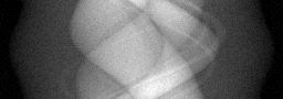
Experimental Setup — Signal Chain

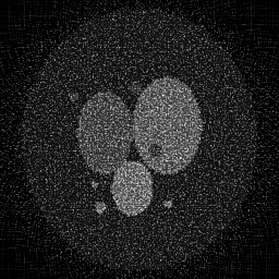
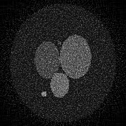
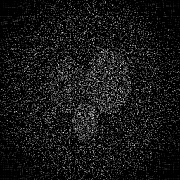
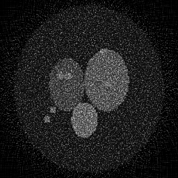
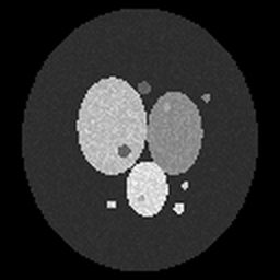
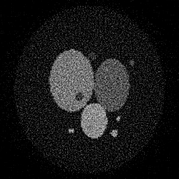
Reconstruction Gallery — 4 Scenes × 3 Scenarios
Method: CPU_baseline | Mismatch: nominal (nominal=True, perturbed=False)

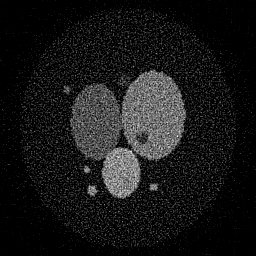
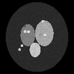
Ground Truth
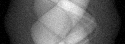
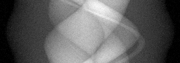
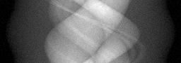
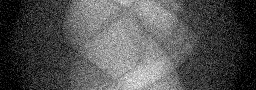
Measurement
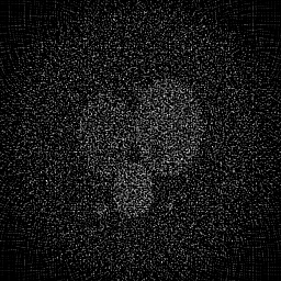
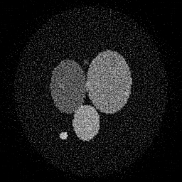
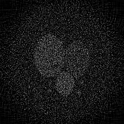
Reconstruction
Ground Truth
Measurement
Reconstruction
Ground Truth
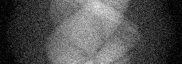
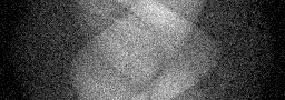
Measurement (perturbed)
Reconstruction


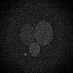

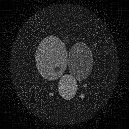
Mean PSNR Across All Scenes
Per-scene PSNR breakdown (4 scenes)
| Scene | I (PSNR) | I (SSIM) | II (PSNR) | II (SSIM) | III (PSNR) | III (SSIM) |
|---|---|---|---|---|---|---|
| scene_00 | 16.584200964385797 | 0.3250905580130585 | 12.506523882319042 | 0.044716474341606735 | 15.931719256055723 | 0.12142227244746187 |
| scene_01 | 18.884299556167566 | 0.3252411352628261 | 13.742128073130111 | 0.048029248758291385 | 17.02391116326154 | 0.11622117666622035 |
| scene_02 | 18.301830801494646 | 0.32976160086547746 | 13.36792873190369 | 0.04964364838717723 | 16.550610792224443 | 0.1259030967011571 |
| scene_03 | 16.67775192548055 | 0.3247822274360334 | 12.53195005733068 | 0.044966709218701925 | 15.850507045662987 | 0.12621817875162467 |
| Mean | 17.61202081188214 | 0.3262188803943489 | 13.037132686170882 | 0.046839020176444326 | 16.33918706430117 | 0.122441181141616 |
Experimental Setup
Key References
- Kardjilov et al., 'Advances in neutron imaging', Materials Today 21, 652-672 (2018)
- IAEA, 'Neutron Imaging: A Non-Destructive Tool for Materials Testing', IAEA-TECDOC-1604 (2008)
Canonical Datasets
- PSI ICON neutron imaging benchmark data
- NIST neutron radiography reference images
Spec DAG — Forward Model Pipeline
R(θ) → Π(neutron) → D(g, η₁)
Mismatch Parameters
| Symbol | Parameter | Description | Nominal | Perturbed |
|---|---|---|---|---|
| ΔE | beam_spectrum | Beam energy spectrum error (%) | 0 | 3.0 |
| Δs | scatter_correction | Scatter correction error (%) | 0 | 5.0 |
| Δθ | rotation_offset | Rotation center offset (pixels) | 0 | 1.0 |
Credits System
Spec Primitives Reference (11 primitives)
Free-space or medium propagation kernel (Fresnel, Rayleigh-Sommerfeld).
Spatial or spatio-temporal amplitude modulation (coded aperture, SLM pattern).
Geometric projection operator (Radon transform, fan-beam, cone-beam).
Sampling in the Fourier / k-space domain (MRI, ptychography).
Shift-invariant convolution with a point-spread function (PSF).
Summation along a physical dimension (spectral, temporal, angular).
Sensor readout with gain g and noise model η (Gaussian, Poisson, mixed).
Patterned illumination (block, Hadamard, random) applied to the scene.
Spectral dispersion element (prism, grating) with shift α and aperture a.
Sample or gantry rotation (CT, electron tomography).
Spectral filter or monochromator selecting a wavelength band.