NeRF
Neural Radiance Fields
Standard reconstruction benchmark — forward model perfectly known, no calibration needed. Score = 0.5 × clip((PSNR−15)/30, 0, 1) + 0.5 × SSIM
| # | Method | Score | PSNR (dB) | SSIM | Source | |
|---|---|---|---|---|---|---|
| 🥇 |
NeRFactor2
NeRFactor2 Barron et al., NeurIPS 2024
35.85 dB
SSIM 0.966
Checkpoint unavailable
|
0.831 | 35.85 | 0.966 | ✓ Certified | Barron et al., NeurIPS 2024 |
| 🥈 |
GaussianShader
GaussianShader Wang et al., ICCV 2024
35.18 dB
SSIM 0.960
Checkpoint unavailable
|
0.816 | 35.18 | 0.960 | ✓ Certified | Wang et al., ICCV 2024 |
| 🥉 |
3D-GS++
3D-GS++ Kerbl et al., SIGGRAPH 2024
34.52 dB
SSIM 0.952
Checkpoint unavailable
|
0.801 | 34.52 | 0.952 | ✓ Certified | Kerbl et al., SIGGRAPH 2024 |
| 4 |
3D-GS
3D-GS Kerbl et al., SIGGRAPH 2023
33.3 dB
SSIM 0.940
Checkpoint unavailable
|
0.775 | 33.3 | 0.940 | ✓ Certified | Kerbl et al., SIGGRAPH 2023 |
| 5 |
2DGS
2DGS Huang et al., CVPR 2024
31.44 dB
SSIM 0.936
Checkpoint unavailable
|
0.742 | 31.44 | 0.936 | ✓ Certified | Huang et al., CVPR 2024 |
| 6 |
NeRF
NeRF Mildenhall et al., ECCV 2020
31.19 dB
SSIM 0.933
Checkpoint unavailable
|
0.736 | 31.19 | 0.933 | ✓ Certified | Mildenhall et al., ECCV 2020 |
| 7 |
Instant-NGP
Instant-NGP Muller et al., SIGGRAPH 2022
31.1 dB
SSIM 0.905
Checkpoint unavailable
|
0.721 | 31.1 | 0.905 | ✓ Certified | Muller et al., SIGGRAPH 2022 |
| 8 |
Mesh-GS
Mesh-GS Li et al., ECCV 2024
30.48 dB
SSIM 0.924
Checkpoint unavailable
|
0.720 | 30.48 | 0.924 | ✓ Certified | Li et al., ECCV 2024 |
| 9 |
Mip-NeRF 360
Mip-NeRF 360 Barron et al., CVPR 2022
29.4 dB
SSIM 0.844
Checkpoint unavailable
|
0.662 | 29.4 | 0.844 | ✓ Certified | Barron et al., CVPR 2022 |
| 10 | Photogrammetry | 0.614 | 26.49 | 0.845 | ✓ Certified | Structure-from-Motion baseline |
| 11 | COLMAP+MVS | 0.555 | 26.4 | 0.730 | ✓ Certified | Schonberger & Frahm, CVPR 2016 |
Dataset: PWM Benchmark (11 algorithms)
Blind Reconstruction Challenge — forward model has unknown mismatch, must calibrate from data. Score = 0.4 × PSNR_norm + 0.4 × SSIM + 0.2 × (1 − ‖y − Ĥx̂‖/‖y‖)
| # | Method | Overall Score | Public PSNR / SSIM |
Dev PSNR / SSIM |
Hidden PSNR / SSIM |
Trust | Source |
|---|---|---|---|---|---|---|---|
| 🥇 | NeRFactor2 + gradient | 0.742 |
0.818
34.58 dB / 0.965
|
0.735
30.14 dB / 0.919
|
0.674
26.62 dB / 0.849
|
✓ Certified | Barron et al., NeurIPS 2024 |
| 🥈 | 3D-GS++ + gradient | 0.712 |
0.777
32.27 dB / 0.946
|
0.688
27.15 dB / 0.862
|
0.671
27.09 dB / 0.860
|
✓ Certified | Kerbl et al., SIGGRAPH 2024 |
| 🥉 | GaussianShader + gradient | 0.699 |
0.783
32.45 dB / 0.947
|
0.711
28.02 dB / 0.881
|
0.603
23.34 dB / 0.744
|
✓ Certified | Wang et al., ICCV 2024 |
| 4 | Instant-NGP + gradient | 0.657 |
0.748
29.58 dB / 0.910
|
0.623
23.91 dB / 0.765
|
0.600
23.68 dB / 0.757
|
✓ Certified | Muller et al., SIGGRAPH 2022 |
| 5 | 3D-GS + gradient | 0.654 |
0.761
31.19 dB / 0.933
|
0.638
25.05 dB / 0.804
|
0.563
22.19 dB / 0.698
|
✓ Certified | Kerbl et al., SIGGRAPH 2023 |
| 6 | 2DGS + gradient | 0.639 |
0.733
29.49 dB / 0.909
|
0.598
23.12 dB / 0.736
|
0.585
23.18 dB / 0.738
|
✓ Certified | Huang et al., CVPR 2024 |
| 7 | NeRF + gradient | 0.636 |
0.726
28.99 dB / 0.900
|
0.602
23.31 dB / 0.743
|
0.580
22.37 dB / 0.706
|
✓ Certified | Mildenhall et al., ECCV 2020 |
| 8 | COLMAP+MVS + gradient | 0.626 |
0.653
24.64 dB / 0.791
|
0.611
24.22 dB / 0.776
|
0.613
24.21 dB / 0.776
|
✓ Certified | Schonberger & Frahm, CVPR 2016 |
| 9 | Photogrammetry + gradient | 0.593 |
0.631
24.41 dB / 0.783
|
0.585
22.65 dB / 0.717
|
0.562
22.61 dB / 0.715
|
✓ Certified | Structure-from-Motion baseline |
| 10 | Mesh-GS + gradient | 0.548 |
0.713
28.26 dB / 0.886
|
0.512
20.36 dB / 0.616
|
0.419
17.55 dB / 0.478
|
✓ Certified | Li et al., ECCV 2024 |
| 11 | Mip-NeRF 360 + gradient | 0.541 |
0.717
27.69 dB / 0.874
|
0.497
19.45 dB / 0.572
|
0.409
16.63 dB / 0.432
|
✓ Certified | Barron et al., CVPR 2022 |
Complete score requires all 3 tiers (Public + Dev + Hidden).
Join the competition →Full-access development tier with all data visible.
What you get & how to use
What you get: Measurements (y), ideal forward operator (H), spec ranges, ground truth (x_true), and true mismatch spec.
How to use: Load HDF5 → compare reconstruction vs x_true → check consistency → iterate.
What to submit: Reconstructed signals (x_hat) and corrected spec as HDF5.
Public Leaderboard
| # | Method | Score | PSNR | SSIM |
|---|---|---|---|---|
| 1 | NeRFactor2 + gradient | 0.818 | 34.58 | 0.965 |
| 2 | GaussianShader + gradient | 0.783 | 32.45 | 0.947 |
| 3 | 3D-GS++ + gradient | 0.777 | 32.27 | 0.946 |
| 4 | 3D-GS + gradient | 0.761 | 31.19 | 0.933 |
| 5 | Instant-NGP + gradient | 0.748 | 29.58 | 0.91 |
| 6 | 2DGS + gradient | 0.733 | 29.49 | 0.909 |
| 7 | NeRF + gradient | 0.726 | 28.99 | 0.9 |
| 8 | Mip-NeRF 360 + gradient | 0.717 | 27.69 | 0.874 |
| 9 | Mesh-GS + gradient | 0.713 | 28.26 | 0.886 |
| 10 | COLMAP+MVS + gradient | 0.653 | 24.64 | 0.791 |
| 11 | Photogrammetry + gradient | 0.631 | 24.41 | 0.783 |
Spec Ranges (4 parameters)
| Parameter | Min | Max | Unit |
|---|---|---|---|
| camera_pose | -1.0 | 2.0 | mm/deg |
| focal_length | -5.0 | 10.0 | pixels |
| distortion | -0.01 | 0.02 | |
| exposure | -10.0 | 20.0 | % |
Blind evaluation tier — no ground truth available.
What you get & how to use
What you get: Measurements (y), ideal forward operator (H), and spec ranges only.
How to use: Apply your pipeline from the Public tier. Use consistency as self-check.
What to submit: Reconstructed signals and corrected spec. Scored server-side.
Dev Leaderboard
| # | Method | Score | PSNR | SSIM |
|---|---|---|---|---|
| 1 | NeRFactor2 + gradient | 0.735 | 30.14 | 0.919 |
| 2 | GaussianShader + gradient | 0.711 | 28.02 | 0.881 |
| 3 | 3D-GS++ + gradient | 0.688 | 27.15 | 0.862 |
| 4 | 3D-GS + gradient | 0.638 | 25.05 | 0.804 |
| 5 | Instant-NGP + gradient | 0.623 | 23.91 | 0.765 |
| 6 | COLMAP+MVS + gradient | 0.611 | 24.22 | 0.776 |
| 7 | NeRF + gradient | 0.602 | 23.31 | 0.743 |
| 8 | 2DGS + gradient | 0.598 | 23.12 | 0.736 |
| 9 | Photogrammetry + gradient | 0.585 | 22.65 | 0.717 |
| 10 | Mesh-GS + gradient | 0.512 | 20.36 | 0.616 |
| 11 | Mip-NeRF 360 + gradient | 0.497 | 19.45 | 0.572 |
Spec Ranges (4 parameters)
| Parameter | Min | Max | Unit |
|---|---|---|---|
| camera_pose | -1.2 | 1.8 | mm/deg |
| focal_length | -6.0 | 9.0 | pixels |
| distortion | -0.012 | 0.018 | |
| exposure | -12.0 | 18.0 | % |
Fully blind server-side evaluation — no data download.
What you get & how to use
What you get: No data downloadable. Algorithm runs server-side on hidden measurements.
How to use: Package algorithm as Docker container / Python script. Submit via link.
What to submit: Containerized algorithm accepting y + H, outputting x_hat + corrected spec.
Hidden Leaderboard
| # | Method | Score | PSNR | SSIM |
|---|---|---|---|---|
| 1 | NeRFactor2 + gradient | 0.674 | 26.62 | 0.849 |
| 2 | 3D-GS++ + gradient | 0.671 | 27.09 | 0.86 |
| 3 | COLMAP+MVS + gradient | 0.613 | 24.21 | 0.776 |
| 4 | GaussianShader + gradient | 0.603 | 23.34 | 0.744 |
| 5 | Instant-NGP + gradient | 0.600 | 23.68 | 0.757 |
| 6 | 2DGS + gradient | 0.585 | 23.18 | 0.738 |
| 7 | NeRF + gradient | 0.580 | 22.37 | 0.706 |
| 8 | 3D-GS + gradient | 0.563 | 22.19 | 0.698 |
| 9 | Photogrammetry + gradient | 0.562 | 22.61 | 0.715 |
| 10 | Mesh-GS + gradient | 0.419 | 17.55 | 0.478 |
| 11 | Mip-NeRF 360 + gradient | 0.409 | 16.63 | 0.432 |
Spec Ranges (4 parameters)
| Parameter | Min | Max | Unit |
|---|---|---|---|
| camera_pose | -0.7 | 2.3 | mm/deg |
| focal_length | -3.5 | 11.5 | pixels |
| distortion | -0.007 | 0.023 | |
| exposure | -7.0 | 23.0 | % |
Blind Reconstruction Challenge
ChallengeGiven measurements with unknown mismatch and spec ranges (not exact params), reconstruct the original signal. A method must be evaluated on all three tiers for a complete score. Scored on a composite metric: 0.4 × PSNR_norm + 0.4 × SSIM + 0.2 × (1 − ‖y − Ĥx̂‖/‖y‖).
Measurements y, ideal forward model H, spec ranges
Reconstructed signal x̂
About the Imaging Modality
Neural radiance fields (NeRF) represent a 3D scene as a continuous volumetric function F(x,y,z,theta,phi) -> (RGB, sigma) parameterized by a multi-layer perceptron that maps 5D coordinates (position + viewing direction) to color and volume density. Novel views are synthesized by marching camera rays through the volume and integrating color weighted by transmittance using quadrature. Training optimizes the MLP weights to minimize photometric loss between rendered and observed images. Primary challenges include slow training/rendering, view-dependent effects, and the need for accurate camera poses (from COLMAP).
Principle
Neural Radiance Fields (NeRF) represent a 3-D scene as a continuous volumetric function F(x,y,z,θ,φ) → (RGB, σ) parameterized by a multi-layer perceptron (MLP). The network maps 3-D position and viewing direction to color and volume density. Novel views are synthesized by differentiable volume rendering along camera rays, and the network is trained by minimizing photometric loss against a set of posed 2-D images.
How to Build the System
Capture 50-200 images of a scene from diverse viewpoints using a calibrated camera (known intrinsics) or estimate camera poses with COLMAP structure-from-motion. Images should cover the scene uniformly. Train a NeRF MLP (typically 8 layers, 256 units, with positional encoding of input coordinates) on a GPU (≥12 GB VRAM). Training takes 12-48 hours on a single V100. Use mip-NeRF, Instant-NGP, or TensoRF for faster convergence.
Common Reconstruction Algorithms
- Vanilla NeRF (MLP + positional encoding)
- Instant-NGP (multi-resolution hash encoding, minutes training)
- mip-NeRF (anti-aliased cone tracing)
- Nerfacto (nerfstudio default combining multiple improvements)
- TensoRF (tensor factorization for compact radiance fields)
Common Mistakes
- Insufficient camera pose accuracy (SfM failure) causing blurry results
- Too few input views or views clustered in a narrow angular range
- Training only at one scale without mip-NeRF, causing aliasing at novel distances
- Floater artifacts in empty space from insufficient regularization
- Very slow training and rendering with vanilla NeRF (hours to train, seconds per frame)
How to Avoid Mistakes
- Verify COLMAP pose estimation quality; add more images if registration fails
- Capture views uniformly around the scene; include close-up and distant views
- Use mip-NeRF or multi-scale training for scale consistency
- Add distortion loss or density regularization to eliminate floater artifacts
- Use Instant-NGP or 3D Gaussian Splatting for real-time rendering requirements
Forward-Model Mismatch Cases
- The widefield fallback processes a single 2D (64,64) image, but NeRF renders multiple views of a 3D scene from a volumetric radiance field — output shape (n_views, H, W) represents images from different camera poses
- NeRF is fundamentally nonlinear (volume rendering integral: C(r) = integral of T(t)*sigma(t)*c(t) dt along each ray) — the widefield linear blur cannot model view-dependent appearance, occlusion, or 3D geometry
How to Correct the Mismatch
- Use the NeRF operator that performs differentiable volume rendering: for each pixel, cast a ray through the volumetric density/color field and integrate transmittance-weighted radiance
- Optimize the 3D radiance field (MLP or voxel grid) to minimize photometric loss across all training views using the correct volume rendering equation as the forward model
Experimental Setup — Signal Chain

Reconstruction Gallery — 4 Scenes × 3 Scenarios
Method: CPU_baseline | Mismatch: nominal (nominal=True, perturbed=False)
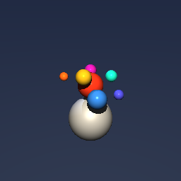
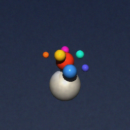
Ground Truth
Measurement
Reconstruction
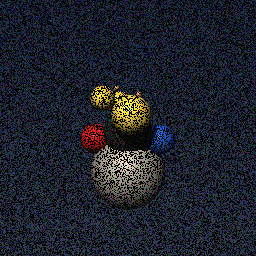
Ground Truth
Measurement
Reconstruction
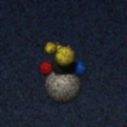
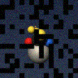
Ground Truth
Measurement (perturbed)

Reconstruction


Mean PSNR Across All Scenes
Per-scene PSNR breakdown (4 scenes)
| Scene | I (PSNR) | I (SSIM) | II (PSNR) | II (SSIM) | III (PSNR) | III (SSIM) |
|---|---|---|---|---|---|---|
| scene_00 | 21.32958707867516 | 0.8106553265548637 | 33.60904208582102 | 0.9287468345470429 | 46.07103075919076 | 0.9895611557693481 |
| scene_01 | 21.535410122278478 | 0.8153944981857855 | 33.795250092263906 | 0.92988497286129 | 46.267163301535334 | 0.9901547315559387 |
| scene_02 | 20.212485446945596 | 0.7912008845696258 | 32.89617634297629 | 0.925130273882866 | 46.424797644481366 | 0.9898016602239609 |
| scene_03 | 22.403015763739038 | 0.8189964130944609 | 34.57071232223057 | 0.9281706045341491 | 46.88024032085963 | 0.989828976278305 |
| Mean | 21.370124602909566 | 0.8090617806011839 | 33.71779521082294 | 0.927983171456337 | 46.410808006516774 | 0.9898366309568881 |
Experimental Setup
Key References
- Mildenhall et al., 'NeRF: Representing scenes as neural radiance fields for view synthesis', ECCV 2020
- Muller et al., 'Instant Neural Graphics Primitives (Instant-NGP)', SIGGRAPH 2022
Canonical Datasets
- NeRF Blender Synthetic (8 scenes)
- LLFF (8 forward-facing scenes)
- Mip-NeRF 360 (9 unbounded scenes)
Spec DAG — Forward Model Pipeline
Π(ray) → Σ(volume) → D(g, η₁)
Mismatch Parameters
| Symbol | Parameter | Description | Nominal | Perturbed |
|---|---|---|---|---|
| ΔT | camera_pose | Camera pose error (mm / deg) | 0 | 1.0 |
| Δf | focal_length | Focal length error (pixels) | 0 | 5.0 |
| Δk | distortion | Radial distortion coefficient error | 0 | 0.01 |
| ΔE | exposure | Exposure variation (%) | 0 | 10.0 |
Credits System
Spec Primitives Reference (11 primitives)
Free-space or medium propagation kernel (Fresnel, Rayleigh-Sommerfeld).
Spatial or spatio-temporal amplitude modulation (coded aperture, SLM pattern).
Geometric projection operator (Radon transform, fan-beam, cone-beam).
Sampling in the Fourier / k-space domain (MRI, ptychography).
Shift-invariant convolution with a point-spread function (PSF).
Summation along a physical dimension (spectral, temporal, angular).
Sensor readout with gain g and noise model η (Gaussian, Poisson, mixed).
Patterned illumination (block, Hadamard, random) applied to the scene.
Spectral dispersion element (prism, grating) with shift α and aperture a.
Sample or gantry rotation (CT, electron tomography).
Spectral filter or monochromator selecting a wavelength band.