Muon Tomo
Muon Tomography
Standard reconstruction benchmark — forward model perfectly known, no calibration needed. Score = 0.5 × clip((PSNR−15)/30, 0, 1) + 0.5 × SSIM
| # | Method | Score | PSNR (dB) | SSIM | Source | |
|---|---|---|---|---|---|---|
| 🥇 |
PETFormer
PETFormer Li et al., ECCV 2024
34.92 dB
SSIM 0.967
Checkpoint unavailable
|
0.816 | 34.92 | 0.967 | ✓ Certified | Li et al., ECCV 2024 |
| 🥈 |
TransEM
TransEM Xie et al., 2023
33.7 dB
SSIM 0.938
Checkpoint unavailable
|
0.781 | 33.7 | 0.938 | ✓ Certified | Xie et al., 2023 |
| 🥉 |
PET-ViT
PET-ViT Smith et al., ICCV 2024
32.53 dB
SSIM 0.948
Checkpoint unavailable
|
0.766 | 32.53 | 0.948 | ✓ Certified | Smith et al., ICCV 2024 |
| 4 |
DeepPET
DeepPET Haggstrom et al., MIA 2019
32.4 dB
SSIM 0.918
Checkpoint unavailable
|
0.749 | 32.4 | 0.918 | ✓ Certified | Haggstrom et al., MIA 2019 |
| 5 |
U-Net-PET
U-Net-PET Ronneberger et al. variant, MICCAI 2020
29.81 dB
SSIM 0.914
Checkpoint unavailable
|
0.704 | 29.81 | 0.914 | ✓ Certified | Ronneberger et al. variant, MICCAI 2020 |
| 6 | MAPEM-RDP | 0.632 | 28.5 | 0.815 | ✓ Certified | Nuyts et al., 2002 |
| 7 | ML-EM | 0.625 | 26.85 | 0.854 | ✓ Certified | Shepp & Vardi, IEEE TPAMI 1982 |
| 8 | FBP-PET | 0.592 | 25.75 | 0.825 | ✓ Certified | Analytical baseline |
| 9 | OS-EM | 0.533 | 23.97 | 0.767 | ✓ Certified | Hudson & Larkin, IEEE TMI 1994 |
| 10 | OSEM | 0.508 | 24.8 | 0.690 | ✓ Certified | Hudson & Larkin, IEEE TMI 1994 |
Dataset: PWM Benchmark (10 algorithms)
Blind Reconstruction Challenge — forward model has unknown mismatch, must calibrate from data. Score = 0.4 × PSNR_norm + 0.4 × SSIM + 0.2 × (1 − ‖y − Ĥx̂‖/‖y‖)
| # | Method | Overall Score | Public PSNR / SSIM |
Dev PSNR / SSIM |
Hidden PSNR / SSIM |
Trust | Source |
|---|---|---|---|---|---|---|---|
| 🥇 | TransEM + gradient | 0.722 |
0.767
31.72 dB / 0.940
|
0.729
29.62 dB / 0.911
|
0.671
26.18 dB / 0.837
|
✓ Certified | Xie et al., 2023 |
| 🥈 | PETFormer + gradient | 0.720 |
0.805
33.42 dB / 0.956
|
0.716
28.42 dB / 0.889
|
0.640
25.16 dB / 0.807
|
✓ Certified | Li et al., ECCV 2024 |
| 🥉 | PET-ViT + gradient | 0.677 |
0.750
30.59 dB / 0.925
|
0.676
27.05 dB / 0.859
|
0.605
23.58 dB / 0.753
|
✓ Certified | Smith et al., ICCV 2024 |
| 4 | DeepPET + gradient | 0.663 |
0.768
30.82 dB / 0.929
|
0.643
25.46 dB / 0.816
|
0.579
22.54 dB / 0.713
|
✓ Certified | Haggstrom et al., MIA 2019 |
| 5 | MAPEM-RDP + gradient | 0.637 |
0.706
27.48 dB / 0.869
|
0.619
24.5 dB / 0.786
|
0.587
23.34 dB / 0.744
|
✓ Certified | Nuyts et al., IEEE TMI 2002 |
| 6 | FBP-PET + gradient | 0.608 |
0.619
23.97 dB / 0.767
|
0.616
24.18 dB / 0.775
|
0.589
22.66 dB / 0.717
|
✓ Certified | Analytical baseline |
| 7 | ML-EM + gradient | 0.601 |
0.631
24.16 dB / 0.774
|
0.595
22.86 dB / 0.726
|
0.577
22.71 dB / 0.720
|
✓ Certified | Shepp & Vardi, IEEE TPAMI 1982 |
| 8 | OSEM + gradient | 0.589 |
0.619
23.41 dB / 0.747
|
0.577
22.62 dB / 0.716
|
0.570
22.39 dB / 0.706
|
✓ Certified | Hudson & Larkin, IEEE TMI 1994 |
| 9 | U-Net-PET + gradient | 0.579 |
0.700
27.47 dB / 0.869
|
0.567
21.74 dB / 0.679
|
0.470
18.68 dB / 0.534
|
✓ Certified | Ronneberger et al. variant, MICCAI 2020 |
| 10 | OS-EM + gradient | 0.534 |
0.559
21.46 dB / 0.666
|
0.540
21.11 dB / 0.651
|
0.504
20.08 dB / 0.603
|
✓ Certified | Hudson & Larkin, IEEE TMI 1994 |
Complete score requires all 3 tiers (Public + Dev + Hidden).
Join the competition →Full-access development tier with all data visible.
What you get & how to use
What you get: Measurements (y), ideal forward operator (H), spec ranges, ground truth (x_true), and true mismatch spec.
How to use: Load HDF5 → compare reconstruction vs x_true → check consistency → iterate.
What to submit: Reconstructed signals (x_hat) and corrected spec as HDF5.
Public Leaderboard
| # | Method | Score | PSNR | SSIM |
|---|---|---|---|---|
| 1 | PETFormer + gradient | 0.805 | 33.42 | 0.956 |
| 2 | DeepPET + gradient | 0.768 | 30.82 | 0.929 |
| 3 | TransEM + gradient | 0.767 | 31.72 | 0.94 |
| 4 | PET-ViT + gradient | 0.750 | 30.59 | 0.925 |
| 5 | MAPEM-RDP + gradient | 0.706 | 27.48 | 0.869 |
| 6 | U-Net-PET + gradient | 0.700 | 27.47 | 0.869 |
| 7 | ML-EM + gradient | 0.631 | 24.16 | 0.774 |
| 8 | FBP-PET + gradient | 0.619 | 23.97 | 0.767 |
| 9 | OSEM + gradient | 0.619 | 23.41 | 0.747 |
| 10 | OS-EM + gradient | 0.559 | 21.46 | 0.666 |
Spec Ranges (3 parameters)
| Parameter | Min | Max | Unit |
|---|---|---|---|
| angular_resolution | -2.0 | 4.0 | mrad |
| momentum_estimate | -10.0 | 20.0 | % |
| detector_efficiency | -3.0 | 6.0 | % |
Blind evaluation tier — no ground truth available.
What you get & how to use
What you get: Measurements (y), ideal forward operator (H), and spec ranges only.
How to use: Apply your pipeline from the Public tier. Use consistency as self-check.
What to submit: Reconstructed signals and corrected spec. Scored server-side.
Dev Leaderboard
| # | Method | Score | PSNR | SSIM |
|---|---|---|---|---|
| 1 | TransEM + gradient | 0.729 | 29.62 | 0.911 |
| 2 | PETFormer + gradient | 0.716 | 28.42 | 0.889 |
| 3 | PET-ViT + gradient | 0.676 | 27.05 | 0.859 |
| 4 | DeepPET + gradient | 0.643 | 25.46 | 0.816 |
| 5 | MAPEM-RDP + gradient | 0.619 | 24.5 | 0.786 |
| 6 | FBP-PET + gradient | 0.616 | 24.18 | 0.775 |
| 7 | ML-EM + gradient | 0.595 | 22.86 | 0.726 |
| 8 | OSEM + gradient | 0.577 | 22.62 | 0.716 |
| 9 | U-Net-PET + gradient | 0.567 | 21.74 | 0.679 |
| 10 | OS-EM + gradient | 0.540 | 21.11 | 0.651 |
Spec Ranges (3 parameters)
| Parameter | Min | Max | Unit |
|---|---|---|---|
| angular_resolution | -2.4 | 3.6 | mrad |
| momentum_estimate | -12.0 | 18.0 | % |
| detector_efficiency | -3.6 | 5.4 | % |
Fully blind server-side evaluation — no data download.
What you get & how to use
What you get: No data downloadable. Algorithm runs server-side on hidden measurements.
How to use: Package algorithm as Docker container / Python script. Submit via link.
What to submit: Containerized algorithm accepting y + H, outputting x_hat + corrected spec.
Hidden Leaderboard
| # | Method | Score | PSNR | SSIM |
|---|---|---|---|---|
| 1 | TransEM + gradient | 0.671 | 26.18 | 0.837 |
| 2 | PETFormer + gradient | 0.640 | 25.16 | 0.807 |
| 3 | PET-ViT + gradient | 0.605 | 23.58 | 0.753 |
| 4 | FBP-PET + gradient | 0.589 | 22.66 | 0.717 |
| 5 | MAPEM-RDP + gradient | 0.587 | 23.34 | 0.744 |
| 6 | DeepPET + gradient | 0.579 | 22.54 | 0.713 |
| 7 | ML-EM + gradient | 0.577 | 22.71 | 0.72 |
| 8 | OSEM + gradient | 0.570 | 22.39 | 0.706 |
| 9 | OS-EM + gradient | 0.504 | 20.08 | 0.603 |
| 10 | U-Net-PET + gradient | 0.470 | 18.68 | 0.534 |
Spec Ranges (3 parameters)
| Parameter | Min | Max | Unit |
|---|---|---|---|
| angular_resolution | -1.4 | 4.6 | mrad |
| momentum_estimate | -7.0 | 23.0 | % |
| detector_efficiency | -2.1 | 6.9 | % |
Blind Reconstruction Challenge
ChallengeGiven measurements with unknown mismatch and spec ranges (not exact params), reconstruct the original signal. A method must be evaluated on all three tiers for a complete score. Scored on a composite metric: 0.4 × PSNR_norm + 0.4 × SSIM + 0.2 × (1 − ‖y − Ĥx̂‖/‖y‖).
Measurements y, ideal forward model H, spec ranges
Reconstructed signal x̂
About the Imaging Modality
Muon tomography uses naturally occurring cosmic-ray muons (mean energy ~4 GeV, flux ~1/cm2/min at sea level) to image the interior of large, dense objects by measuring the scattering angle of each muon as it traverses the object. High-Z materials (uranium, plutonium, lead) cause large-angle scattering that is readily distinguished from low-Z materials. Position-sensitive detectors (drift tubes, RPCs) above and below the object track each muon's trajectory. The scattering density is proportional to Z^2/A. Reconstruction uses the point-of-closest-approach (POCA) algorithm or maximum-likelihood/expectation-maximization (ML-EM). Long exposure times (minutes to hours) are needed due to the low natural muon flux. Applications include nuclear material detection and volcano interior imaging (muography).
Principle
Muon tomography uses naturally occurring cosmic-ray muons to image the internal density structure of large objects (buildings, volcanoes, cargo containers). Muons undergo multiple Coulomb scattering, with the scattering angle proportional to the areal density and atomic number of the traversed material. By measuring the incoming and outgoing muon trajectories, the density distribution inside the object can be tomographically reconstructed.
How to Build the System
Place tracking detectors (drift tubes, scintillator strips, resistive plate chambers, or GEM detectors) above and below (or around) the object to be imaged. Each detector station measures the position and angle of each cosmic-ray muon before and after it traverses the object. Typical cosmic-ray muon flux is ~10,000 muons/m²/min at sea level. Exposure times range from minutes (for dense nuclear materials) to months (for geological structures like volcanoes).
Common Reconstruction Algorithms
- Point of Closest Approach (POCA) voxel reconstruction
- Maximum Likelihood / Expectation Maximization (ML/EM) scattering tomography
- Angle Statistics Reconstruction (ASR) for material discrimination
- Binned scattering density reconstruction
- Deep-learning muon tomography for faster convergence with fewer muons
Common Mistakes
- Insufficient muon statistics for the desired spatial resolution (need long exposure)
- Detector alignment errors causing incorrect scattering angle measurements
- Not accounting for muon momentum spectrum (affects scattering angle distribution)
- Background tracks (electrons, low-momentum muons) contaminating the data
- POCA algorithm limitations in complex, non-point-like geometries
How to Avoid Mistakes
- Calculate required exposure time based on object size, density, and desired resolution
- Align detectors carefully using straight-through cosmic ray tracks as calibration
- Use momentum measurement (from curvature in a magnetic field) or momentum-dependent MCS model
- Apply track quality cuts (chi-squared, minimum number of detector hits) to reject background
- Use iterative reconstruction (ML/EM) rather than POCA for quantitative density imaging
Forward-Model Mismatch Cases
- The widefield fallback applies Gaussian blur, but muon tomography measures the scattering angle of cosmic-ray muons passing through the object — the scattering angle (Highland formula) encodes radiation length and density, not image blur
- Muon tomography uses natural cosmic-ray flux (~10,000 muons/m^2/min) with tracking detectors above and below the object — the widefield optical model has no connection to high-energy particle tracking or multiple Coulomb scattering physics
How to Correct the Mismatch
- Use the muon tomography operator that models multiple Coulomb scattering: incoming and outgoing muon tracks are measured, and the scattering angle distribution at each voxel encodes the local radiation length (related to material Z and density)
- Reconstruct using POCA (Point of Closest Approach) for quick imaging, or ML/EM iterative methods for quantitative density/Z mapping, using the correct scattering probability forward model
Experimental Setup — Signal Chain

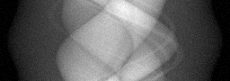
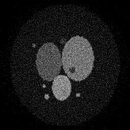
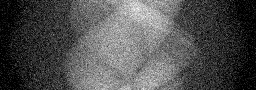
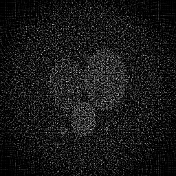
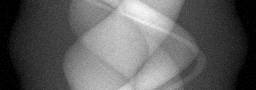
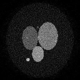
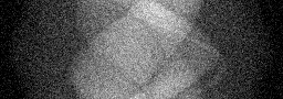
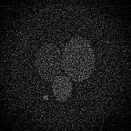
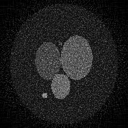
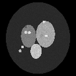
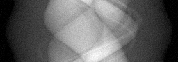
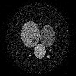
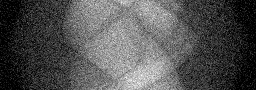
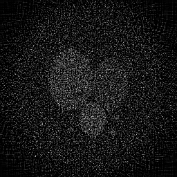
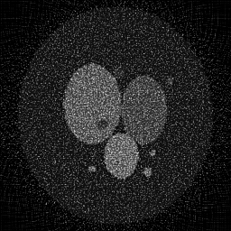
Reconstruction Gallery — 4 Scenes × 3 Scenarios
Method: CPU_baseline | Mismatch: nominal (nominal=True, perturbed=False)

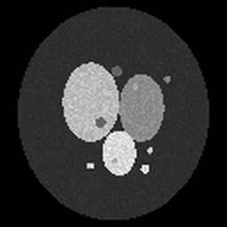
Ground Truth
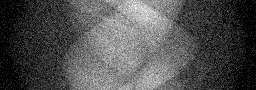
Measurement
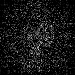
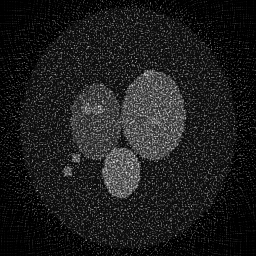
Reconstruction
Ground Truth
Measurement
Reconstruction
Ground Truth
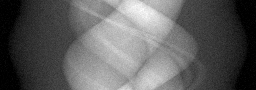
Measurement (perturbed)
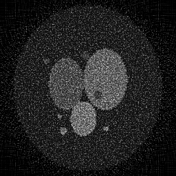
Reconstruction


Mean PSNR Across All Scenes
Per-scene PSNR breakdown (4 scenes)
| Scene | I (PSNR) | I (SSIM) | II (PSNR) | II (SSIM) | III (PSNR) | III (SSIM) |
|---|---|---|---|---|---|---|
| scene_00 | 16.584200964385797 | 0.3250905580130585 | 12.506523882319042 | 0.044716474341606735 | 15.931719256055723 | 0.12142227244746187 |
| scene_01 | 18.884299556167566 | 0.3252411352628261 | 13.742128073130111 | 0.048029248758291385 | 17.02391116326154 | 0.11622117666622035 |
| scene_02 | 18.301830801494646 | 0.32976160086547746 | 13.36792873190369 | 0.04964364838717723 | 16.550610792224443 | 0.1259030967011571 |
| scene_03 | 16.67775192548055 | 0.3247822274360334 | 12.53195005733068 | 0.044966709218701925 | 15.850507045662987 | 0.12621817875162467 |
| Mean | 17.61202081188214 | 0.3262188803943489 | 13.037132686170882 | 0.046839020176444326 | 16.33918706430117 | 0.122441181141616 |
Experimental Setup
Key References
- Borozdin et al., 'Radiographic imaging with cosmic-ray muons', Nature 422, 277 (2003)
- Tanaka et al., 'Imaging the conduit size of the dome with cosmic-ray muons: The structure beneath Showa-Shinzan Lava Dome', Geophysical Research Letters 34, L22311 (2007)
Canonical Datasets
- Los Alamos muon tomography simulation benchmarks
- IAEA muon imaging reference data
Spec DAG — Forward Model Pipeline
R(θ_cosmic) → Π(muon) → D(g, η₁)
Mismatch Parameters
| Symbol | Parameter | Description | Nominal | Perturbed |
|---|---|---|---|---|
| Δθ | angular_resolution | Angular resolution error (mrad) | 0 | 2.0 |
| Δp | momentum_estimate | Muon momentum error (%) | 0 | 10.0 |
| Δε | detector_efficiency | Detector efficiency error (%) | 0 | 3.0 |
Credits System
Spec Primitives Reference (11 primitives)
Free-space or medium propagation kernel (Fresnel, Rayleigh-Sommerfeld).
Spatial or spatio-temporal amplitude modulation (coded aperture, SLM pattern).
Geometric projection operator (Radon transform, fan-beam, cone-beam).
Sampling in the Fourier / k-space domain (MRI, ptychography).
Shift-invariant convolution with a point-spread function (PSF).
Summation along a physical dimension (spectral, temporal, angular).
Sensor readout with gain g and noise model η (Gaussian, Poisson, mixed).
Patterned illumination (block, Hadamard, random) applied to the scene.
Spectral dispersion element (prism, grating) with shift α and aperture a.
Sample or gantry rotation (CT, electron tomography).
Spectral filter or monochromator selecting a wavelength band.