MRS
MR Spectroscopy
Standard reconstruction benchmark — forward model perfectly known, no calibration needed. Score = 0.5 × clip((PSNR−15)/30, 0, 1) + 0.5 × SSIM
| # | Method | Score | PSNR (dB) | SSIM | Source | |
|---|---|---|---|---|---|---|
| 🥇 |
SwinMR++
SwinMR++ Huang et al., IEEE TMI 2025 — 5 improvements: multi-scale axial attention (cross-scale long-range modeling), INR coordinate-query head (high-acceleration k-space interpolation), k-space DC per unrolled module, joint LPIPS+SSIM+k-space consistency loss, dynamic conv-Transformer branch weighting
43.8 dB
SSIM 0.983
Checkpoint unavailable
|
0.971 | 43.8 | 0.983 | ✓ Certified | Huang et al., IEEE TMI 2025 — 5 improvements: multi-scale axial attention (cross-scale long-range modeling), INR coordinate-query head (high-acceleration k-space interpolation), k-space DC per unrolled module, joint LPIPS+SSIM+k-space consistency loss, dynamic conv-Transformer branch weighting |
| 🥈 |
HUMUS-Net++
HUMUS-Net++ Fabian et al., dHUMUS-Net 2023 — 5 improvements: k-space DC per unrolled module, dynamic optimal-scale prediction (dHUMUS-Net), INR coordinate head (continuous representation), LPIPS+SSIM perceptual-structural loss, lightweight axial attention Transformer
43.1 dB
SSIM 0.979
Checkpoint unavailable
|
0.958 | 43.1 | 0.979 | ✓ Certified | Fabian et al., dHUMUS-Net 2023 — 5 improvements: k-space DC per unrolled module, dynamic optimal-scale prediction (dHUMUS-Net), INR coordinate head (continuous representation), LPIPS+SSIM perceptual-structural loss, lightweight axial attention Transformer |
| 🥉 |
MR-IPT
MR-IPT Sci. Reports 2025
42.48 dB
SSIM 0.983
Checkpoint unavailable
|
0.950 | 42.48 | 0.983 | ✓ Certified | Sci. Reports 2025 |
| 4 |
HybridCascade++
HybridCascade++ HybridCascade++ MICCAI 2021 + IEEE TMI 2025 — 5 improvements: multi-stage cascade DC (coarse-to-fine 4-stage unrolling), SIREN INR warm-start (continuous prior initialization), SSIM structural anchor (perceptual consistency in late DC stages), DRUNet final polish (blind denoising post-DC), freq-blend LF/HF fusion (SIREN low-freq + structured high-freq recombination)
42.5 dB
SSIM 0.981
Checkpoint unavailable
|
0.949 | 42.5 | 0.981 | ✓ Certified | HybridCascade++ MICCAI 2021 + IEEE TMI 2025 — 5 improvements: multi-stage cascade DC (coarse-to-fine 4-stage unrolling), SIREN INR warm-start (continuous prior initialization), SSIM structural anchor (perceptual consistency in late DC stages), DRUNet final polish (blind denoising post-DC), freq-blend LF/HF fusion (SIREN low-freq + structured high-freq recombination) |
| 5 |
MoDL-Net++
MoDL-Net++ MoDL-Net++ IEEE TMI 2025 — 5 improvements: multi-scale pyramid fusion (coarse-to-fine representation), RDN/Swin deep prior (rich feature hierarchy), differentiable DC layers (physics-informed unrolling), joint LPIPS+SSIM+L1 loss (perceptual+structural+fidelity), two-stage training (pre-train then fine-tune with DC)
41.8 dB
SSIM 0.978
Checkpoint unavailable
|
0.936 | 41.8 | 0.978 | ✓ Certified | MoDL-Net++ IEEE TMI 2025 — 5 improvements: multi-scale pyramid fusion (coarse-to-fine representation), RDN/Swin deep prior (rich feature hierarchy), differentiable DC layers (physics-informed unrolling), joint LPIPS+SSIM+L1 loss (perceptual+structural+fidelity), two-stage training (pre-train then fine-tune with DC) |
| 6 |
U-Net++
U-Net++ Chen & Boning, IEEE TMI 2024 — 5 improvements: Residual U-Net blocks (dense skip connections), data consistency layers (physics-informed k-space projection), plug-and-play prior (learned denoiser as proximal operator), joint SSIM+MSE+DC loss, multi-scale feature aggregation
41.5 dB
SSIM 0.978
Checkpoint unavailable
|
0.931 | 41.5 | 0.978 | ✓ Certified | Chen & Boning, IEEE TMI 2024 — 5 improvements: Residual U-Net blocks (dense skip connections), data consistency layers (physics-informed k-space projection), plug-and-play prior (learned denoiser as proximal operator), joint SSIM+MSE+DC loss, multi-scale feature aggregation |
| 7 |
MRI-FM
MRI-FM Wang et al., Nature MI 2026
42.1 dB
SSIM 0.948
Checkpoint unavailable
|
0.926 | 42.1 | 0.948 | ✓ Certified | Wang et al., Nature MI 2026 |
| 8 |
ReconFormer++
ReconFormer++ Pan et al., IEEE TMI 2025
41.5 dB
SSIM 0.969
Checkpoint unavailable
|
0.926 | 41.5 | 0.969 | ✓ Certified | Pan et al., IEEE TMI 2025 |
| 9 |
PromptMR-SFM
PromptMR-SFM PWM 2026
41.3 dB
SSIM 0.971
Checkpoint unavailable
|
0.924 | 41.3 | 0.971 | ✓ Certified | PWM 2026 |
| 10 |
PnP-DnCNN-Pro
PnP-DnCNN-Pro PnP-DnCNN-Pro IEEE TMI 2025 (DOI:10.1109/TMI.2025.3441240) — 5 improvements: multi-scale DnCNN denoiser (SwinIR-style hierarchical feature extraction), adaptive mu/sigma schedule (dynamic regularization per PnP iteration), SIREN INR coordinate output head (continuous representation for high-acceleration interpolation), joint LPIPS+SSIM denoiser training (perceptual+structural loss), dynamic PnP regularization scheduling (learnable lambda per iteration)
41.0 dB
SSIM 0.968
Try in SpecLab →
|
0.917 | 41.0 | 0.968 | ✓ Certified | PnP-DnCNN-Pro IEEE TMI 2025 (DOI:10.1109/TMI.2025.3441240) — 5 improvements: multi-scale DnCNN denoiser (SwinIR-style hierarchical feature extraction), adaptive mu/sigma schedule (dynamic regularization per PnP iteration), SIREN INR coordinate output head (continuous representation for high-acceleration interpolation), joint LPIPS+SSIM denoiser training (perceptual+structural loss), dynamic PnP regularization scheduling (learnable lambda per iteration) |
| 11 |
MMR-Mamba
MMR-Mamba Zhao et al., Med. Image Anal. 2025
40.98 dB
SSIM 0.969
Checkpoint unavailable
|
0.917 | 40.98 | 0.969 | ✓ Certified | Zhao et al., Med. Image Anal. 2025 |
| 12 |
BrainID-MRI
BrainID-MRI Liu et al., CVPR 2025
41.0 dB
SSIM 0.942
Checkpoint unavailable
|
0.904 | 41.0 | 0.942 | ✓ Certified | Liu et al., CVPR 2025 |
| 13 |
MRDynamo
MRDynamo Chen et al., NeurIPS 2024
40.5 dB
SSIM 0.938
Checkpoint unavailable
|
0.894 | 40.5 | 0.938 | ✓ Certified | Chen et al., NeurIPS 2024 |
| 14 |
MRI-DiffusionNet
MRI-DiffusionNet Song et al., ICCV 2024
40.1 dB
SSIM 0.932
Checkpoint unavailable
|
0.884 | 40.1 | 0.932 | ✓ Certified | Song et al., ICCV 2024 |
| 15 |
PromptMR
PromptMR Bai et al., ECCV 2024
39.7 dB
SSIM 0.926
Checkpoint unavailable
|
0.875 | 39.7 | 0.926 | ✓ Certified | Bai et al., ECCV 2024 |
| 16 |
E2E-VarNet
E2E-VarNet Sriram et al., MICCAI 2020
39.4 dB
SSIM 0.924
Checkpoint unavailable
|
0.869 | 39.4 | 0.924 | ✓ Certified | Sriram et al., MICCAI 2020 |
| 17 |
ReconFormer
ReconFormer Guo et al., IEEE TMI 2024
39.0 dB
SSIM 0.922
Checkpoint unavailable
|
0.861 | 39.0 | 0.922 | ✓ Certified | Guo et al., IEEE TMI 2024 |
| 18 |
HUMUS-Net
HUMUS-Net Fabian et al., NeurIPS 2022
38.9 dB
SSIM 0.923
Checkpoint unavailable
|
0.860 | 38.9 | 0.923 | ✓ Certified | Fabian et al., NeurIPS 2022 |
| 19 |
SwinMR
SwinMR Huang et al., MICCAI 2022
38.5 dB
SSIM 0.921
Checkpoint unavailable
|
0.852 | 38.5 | 0.921 | ✓ Certified | Huang et al., MICCAI 2022 |
| 20 |
HybridCascade
HybridCascade Fastmri, arXiv 2020
37.8 dB
SSIM 0.917
Checkpoint unavailable
|
0.839 | 37.8 | 0.917 | ✓ Certified | Fastmri, arXiv 2020 |
| 21 |
MoDL
MoDL Aggarwal et al., IEEE TMI 2019
36.5 dB
SSIM 0.912
Checkpoint unavailable
|
0.814 | 36.5 | 0.912 | ✓ Certified | Aggarwal et al., IEEE TMI 2019 |
| 22 |
U-Net
U-Net Zbontar et al., arXiv 2018
35.9 dB
SSIM 0.904
Checkpoint unavailable
|
0.800 | 35.9 | 0.904 | ✓ Certified | Zbontar et al., arXiv 2018 |
| 23 |
DCCNN
DCCNN Schlemper et al., IEEE TMI 2018
35.5 dB
SSIM 0.908
Checkpoint unavailable
|
0.796 | 35.5 | 0.908 | ✓ Certified | Schlemper et al., IEEE TMI 2018 |
| 24 |
Deep-ADMM-Net
Deep-ADMM-Net Yang et al., NeurIPS 2016
35.3 dB
SSIM 0.907
Checkpoint unavailable
|
0.792 | 35.3 | 0.907 | ✓ Certified | Yang et al., NeurIPS 2016 |
| 25 |
PnP-DnCNN
PnP-DnCNN Ahmad et al., IEEE TCI 2019 (DOI:10.1109/TCI.2019.2944521)
35.0 dB
SSIM 0.905
Try in SpecLab →
|
0.786 | 35.0 | 0.905 | ✓ Certified | Ahmad et al., IEEE TCI 2019 (DOI:10.1109/TCI.2019.2944521) |
| 26 | ALOHA | 0.775 | 34.5 | 0.900 | ✓ Certified | Jin et al., IEEE TMI 2016 |
| 27 | BM3D-MRI | 0.769 | 34.2 | 0.897 | ✓ Certified | Eksioglu, Comput. Math. Meth. Med. 2016 |
| 28 | LORAKS | 0.760 | 33.8 | 0.893 | ✓ Certified | Haldar, IEEE TMI 2014 |
| 29 | ESPIRiT | 0.752 | 33.4 | 0.890 | ✓ Certified | Uecker et al., MRM 2014 |
| 30 | k-t SPARSE-SENSE | 0.729 | 32.5 | 0.875 | ✓ Certified | Lustig et al., MRM 2006 |
| 31 | L1-Wavelet | 0.720 | 32.1 | 0.870 | ✓ Certified | Lustig et al., MRM 2007 |
| 32 |
Score-MRI
Score-MRI Chung & Ye, Med. Image Anal. 2022
31.4 dB
SSIM 0.890
Checkpoint unavailable
|
0.718 | 31.4 | 0.890 | ✓ Certified | Chung & Ye, Med. Image Anal. 2022 |
| 33 | GRAPPA | 0.700 | 31.2 | 0.860 | ✓ Certified | Griswold et al., MRM 2002 |
| 34 | SENSE | 0.657 | 29.5 | 0.830 | ✓ Certified | Pruessmann et al., MRM 1999 |
| 35 | Zero-Filled IFFT | 0.493 | 26.0 | 0.620 | ✓ Certified | Pruessmann et al., MRM 1999 |
Dataset: PWM Benchmark (35 algorithms)
Blind Reconstruction Challenge — forward model has unknown mismatch, must calibrate from data. Score = 0.4 × PSNR_norm + 0.4 × SSIM + 0.2 × (1 − ‖y − Ĥx̂‖/‖y‖)
| # | Method | Overall Score | Public PSNR / SSIM |
Dev PSNR / SSIM |
Hidden PSNR / SSIM |
Trust | Source |
|---|---|---|---|---|---|---|---|
| 🥇 |
SwinMR++ + gradient
SwinMR++ + gradient Huang et al., IEEE TMI 2025 — multi-scale axial attention + INR head + k-space DC per module + LPIPS+SSIM+k-space joint loss + dynamic feature fusion Score 0.848
Correct & Reconstruct →
|
0.848 |
0.908
42.34 dB / 0.992
|
0.837
37.32 dB / 0.979
|
0.798
34.26 dB / 0.963
|
✓ Certified | Huang et al., IEEE TMI 2025 — multi-scale axial attention + INR head + k-space DC per module + LPIPS+SSIM+k-space joint loss + dynamic feature fusion |
| 🥈 |
PnP-DnCNN-Pro + gradient
PnP-DnCNN-Pro + gradient PnP-DnCNN-Pro IEEE TMI 2025 (DOI:10.1109/TMI.2025.3441240) — multi-scale DnCNN denoiser + adaptive mu/sigma schedule + SIREN INR output head + joint LPIPS+SSIM denoiser training + dynamic PnP regularization scheduling Score 0.846
Correct & Reconstruct →
|
0.846 |
0.877
39.62 dB / 0.987
|
0.842
38.09 dB / 0.982
|
0.820
35.72 dB / 0.972
|
✓ Certified | PnP-DnCNN-Pro IEEE TMI 2025 (DOI:10.1109/TMI.2025.3441240) — multi-scale DnCNN denoiser + adaptive mu/sigma schedule + SIREN INR output head + joint LPIPS+SSIM denoiser training + dynamic PnP regularization scheduling |
| 🥉 |
HUMUS-Net++ + gradient
HUMUS-Net++ + gradient Fabian et al., dHUMUS-Net 2023 — k-space DC per module + dynamic multi-scale weighting + INR head + perceptual-structural loss + axial attention Score 0.838
Correct & Reconstruct →
|
0.838 |
0.900
41.55 dB / 0.991
|
0.840
37.74 dB / 0.981
|
0.775
33.17 dB / 0.954
|
✓ Certified | Fabian et al., dHUMUS-Net 2023 — k-space DC per module + dynamic multi-scale weighting + INR head + perceptual-structural loss + axial attention |
| 4 | ReconFormer++ + gradient | 0.835 |
0.862
39.19 dB / 0.986
|
0.841
36.99 dB / 0.978
|
0.801
35.47 dB / 0.971
|
✓ Certified | Pan et al., IEEE TMI 2025 |
| 5 |
HybridCascade++ + gradient
HybridCascade++ + gradient HybridCascade++ MICCAI 2021 + IEEE TMI 2025 — multi-scale cascade DC + SIREN INR warm-start + SSIM structural anchor + DRUNet polish + freq-blend LF/HF fusion Score 0.833
Correct & Reconstruct →
|
0.833 |
0.894
41.03 dB / 0.990
|
0.817
35.0 dB / 0.968
|
0.787
33.14 dB / 0.954
|
✓ Certified | HybridCascade++ MICCAI 2021 + IEEE TMI 2025 — multi-scale cascade DC + SIREN INR warm-start + SSIM structural anchor + DRUNet polish + freq-blend LF/HF fusion |
| 6 | MR-IPT + gradient | 0.829 |
0.894
41.16 dB / 0.990
|
0.810
35.74 dB / 0.972
|
0.784
34.24 dB / 0.963
|
✓ Certified | Sci. Reports 2025 |
| 7 | BrainID-MRI + gradient | 0.808 |
0.858
39.2 dB / 0.986
|
0.789
34.51 dB / 0.964
|
0.776
32.31 dB / 0.946
|
✓ Certified | Liu et al., CVPR 2025 |
| 8 | MRI-FM + gradient | 0.807 |
0.871
40.31 dB / 0.989
|
0.797
34.53 dB / 0.965
|
0.752
32.2 dB / 0.945
|
✓ Certified | Wang et al., Nature MI 2026 |
| 9 | MRDynamo + gradient | 0.793 |
0.853
38.57 dB / 0.984
|
0.777
33.58 dB / 0.958
|
0.748
32.04 dB / 0.943
|
✓ Certified | Chen et al., NeurIPS 2024 |
| 10 | ReconFormer + gradient | 0.791 |
0.855
37.81 dB / 0.981
|
0.780
32.76 dB / 0.950
|
0.739
30.02 dB / 0.917
|
✓ Certified | Guo et al., IEEE TMI 2024 |
| 11 |
MoDL-Net++ + gradient
MoDL-Net++ + gradient MoDL-Net++ IEEE TMI 2025 — multi-scale pyramid fusion + RDN/Swin deep prior + differentiable DC layers + LPIPS+SSIM+L1 joint loss + two-stage training strategy Score 0.786
Correct & Reconstruct →
|
0.786 |
0.868
39.48 dB / 0.987
|
0.753
31.89 dB / 0.941
|
0.737
30.49 dB / 0.924
|
✓ Certified | MoDL-Net++ IEEE TMI 2025 — multi-scale pyramid fusion + RDN/Swin deep prior + differentiable DC layers + LPIPS+SSIM+L1 joint loss + two-stage training strategy |
| 12 | MMR-Mamba + gradient | 0.784 |
0.858
39.15 dB / 0.986
|
0.765
31.71 dB / 0.939
|
0.728
29.32 dB / 0.906
|
✓ Certified | Zhao et al., Med. Image Anal. 2025 |
| 13 |
U-Net++ + gradient
U-Net++ + gradient Chen & Boning, IEEE TMI 2024 (DOI: 10.1109/TMI.2024.3367890) — Residual U-Net + data consistency layers + plug-and-play prior + residual connections + dense skip paths Score 0.779
Correct & Reconstruct →
|
0.779 |
0.885
40.49 dB / 0.989
|
0.761
31.31 dB / 0.935
|
0.690
28.4 dB / 0.889
|
✓ Certified | Chen & Boning, IEEE TMI 2024 (DOI: 10.1109/TMI.2024.3367890) — Residual U-Net + data consistency layers + plug-and-play prior + residual connections + dense skip paths |
| 14 | SwinMR + gradient | 0.775 |
0.849
36.95 dB / 0.978
|
0.758
32.05 dB / 0.943
|
0.718
29.35 dB / 0.906
|
✓ Certified | Huang et al., MICCAI 2022 |
| 15 | MRI-DiffusionNet + gradient | 0.775 |
0.848
37.76 dB / 0.981
|
0.752
31.54 dB / 0.937
|
0.726
29.93 dB / 0.916
|
✓ Certified | Song et al., ICCV 2024 |
| 16 | PromptMR + gradient | 0.773 |
0.862
38.31 dB / 0.983
|
0.749
31.18 dB / 0.933
|
0.709
28.37 dB / 0.888
|
✓ Certified | Bai et al., ECCV 2024 |
| 17 | PromptMR-SFM + gradient | 0.772 |
0.863
39.41 dB / 0.986
|
0.759
31.69 dB / 0.939
|
0.695
28.62 dB / 0.893
|
✓ Certified | PWM 2026 |
| 18 | E2E-VarNet + gradient | 0.764 |
0.837
36.65 dB / 0.977
|
0.754
30.46 dB / 0.924
|
0.702
28.55 dB / 0.892
|
✓ Certified | Sriram et al., MICCAI 2020 |
| 19 | HUMUS-Net + gradient | 0.758 |
0.834
36.72 dB / 0.977
|
0.755
30.75 dB / 0.928
|
0.685
28.17 dB / 0.884
|
✓ Certified | Fabian et al., NeurIPS 2022 |
| 20 |
PnP-DnCNN + gradient
PnP-DnCNN + gradient Ahmad et al., IEEE TCI 2019 (DOI:10.1109/TCI.2019.2944521) Score 0.745
Correct & Reconstruct →
|
0.745 |
0.805
33.46 dB / 0.957
|
0.738
29.44 dB / 0.908
|
0.692
27.48 dB / 0.869
|
✓ Certified | Ahmad et al., IEEE TCI 2019 (DOI:10.1109/TCI.2019.2944521) |
| 21 | BM3D-MRI + gradient | 0.737 |
0.771
31.62 dB / 0.938
|
0.728
29.12 dB / 0.902
|
0.713
29.04 dB / 0.901
|
✓ Certified | Eksioglu, Comput. Math. Meth. Med. 2016 |
| 22 | MoDL + gradient | 0.728 |
0.827
35.47 dB / 0.971
|
0.696
28.28 dB / 0.887
|
0.662
25.88 dB / 0.829
|
✓ Certified | Aggarwal et al., IEEE TMI 2019 |
| 23 | Deep-ADMM-Net + gradient | 0.725 |
0.808
33.66 dB / 0.958
|
0.696
27.47 dB / 0.869
|
0.671
27.09 dB / 0.860
|
✓ Certified | Yang et al., NeurIPS 2016 |
| 24 | GRAPPA + gradient | 0.721 |
0.729
29.26 dB / 0.905
|
0.712
29.24 dB / 0.904
|
0.723
29.51 dB / 0.909
|
✓ Certified | Griswold et al., MRM 2002 |
| 25 | U-Net + gradient | 0.720 |
0.818
34.8 dB / 0.966
|
0.694
27.16 dB / 0.862
|
0.647
25.72 dB / 0.824
|
✓ Certified | Zbontar et al., arXiv 2018 |
| 26 | HybridCascade + gradient | 0.719 |
0.821
35.81 dB / 0.972
|
0.691
27.29 dB / 0.865
|
0.645
25.27 dB / 0.811
|
✓ Certified | Fastmri, arXiv 2020 |
| 27 | DCCNN + gradient | 0.712 |
0.811
33.78 dB / 0.959
|
0.697
27.73 dB / 0.875
|
0.629
24.33 dB / 0.780
|
✓ Certified | Schlemper et al., IEEE TMI 2018 |
| 28 | ALOHA + gradient | 0.705 |
0.778
32.52 dB / 0.948
|
0.709
28.38 dB / 0.889
|
0.629
25.38 dB / 0.814
|
✓ Certified | Jin et al., IEEE TMI 2016 |
| 29 | ESPIRiT + gradient | 0.679 |
0.787
32.37 dB / 0.947
|
0.670
26.34 dB / 0.841
|
0.579
22.65 dB / 0.717
|
✓ Certified | Uecker et al., MRM 2014 |
| 30 | LORAKS + gradient | 0.670 |
0.789
32.27 dB / 0.946
|
0.647
25.36 dB / 0.813
|
0.575
22.95 dB / 0.729
|
✓ Certified | Haldar, IEEE TMI 2014 |
| 31 | SENSE + gradient | 0.666 |
0.718
27.79 dB / 0.876
|
0.665
25.63 dB / 0.821
|
0.614
24.43 dB / 0.783
|
✓ Certified | Pruessmann et al., MRM 1999 |
| 32 | L1-Wavelet + gradient | 0.639 |
0.740
29.67 dB / 0.912
|
0.640
25.07 dB / 0.804
|
0.537
21.03 dB / 0.647
|
✓ Certified | Lustig et al., MRM 2007 |
| 33 | k-t SPARSE-SENSE + gradient | 0.621 |
0.746
30.2 dB / 0.920
|
0.584
22.36 dB / 0.705
|
0.532
20.99 dB / 0.645
|
✓ Certified | Lustig et al., MRM 2006 |
| 34 | Score-MRI + gradient | 0.618 |
0.726
28.64 dB / 0.894
|
0.596
23.46 dB / 0.749
|
0.533
21.52 dB / 0.669
|
✓ Certified | Chung & Ye, Med. Image Anal. 2022 |
| 35 | Zero-Filled IFFT + gradient | 0.616 |
0.621
23.97 dB / 0.767
|
0.628
24.54 dB / 0.787
|
0.598
23.55 dB / 0.752
|
✓ Certified | Pruessmann et al., MRM 1999 |
Complete score requires all 3 tiers (Public + Dev + Hidden).
Join the competition →Full-access development tier with all data visible.
What you get & how to use
What you get: Measurements (y), ideal forward operator (H), spec ranges, ground truth (x_true), and true mismatch spec.
How to use: Load HDF5 → compare reconstruction vs x_true → check consistency → iterate.
What to submit: Reconstructed signals (x_hat) and corrected spec as HDF5.
Public Leaderboard
| # | Method | Score | PSNR | SSIM |
|---|---|---|---|---|
| 1 | SwinMR++ + gradient | 0.908 | 42.34 | 0.992 |
| 2 | HUMUS-Net++ + gradient | 0.900 | 41.55 | 0.991 |
| 3 | HybridCascade++ + gradient | 0.894 | 41.03 | 0.99 |
| 4 | MR-IPT + gradient | 0.894 | 41.16 | 0.99 |
| 5 | U-Net++ + gradient | 0.885 | 40.49 | 0.989 |
| 6 | PnP-DnCNN-Pro + gradient | 0.877 | 39.62 | 0.987 |
| 7 | MRI-FM + gradient | 0.871 | 40.31 | 0.989 |
| 8 | MoDL-Net++ + gradient | 0.868 | 39.48 | 0.987 |
| 9 | PromptMR-SFM + gradient | 0.863 | 39.41 | 0.986 |
| 10 | ReconFormer++ + gradient | 0.862 | 39.19 | 0.986 |
| 11 | PromptMR + gradient | 0.862 | 38.31 | 0.983 |
| 12 | BrainID-MRI + gradient | 0.858 | 39.2 | 0.986 |
| 13 | MMR-Mamba + gradient | 0.858 | 39.15 | 0.986 |
| 14 | ReconFormer + gradient | 0.855 | 37.81 | 0.981 |
| 15 | MRDynamo + gradient | 0.853 | 38.57 | 0.984 |
| 16 | SwinMR + gradient | 0.849 | 36.95 | 0.978 |
| 17 | MRI-DiffusionNet + gradient | 0.848 | 37.76 | 0.981 |
| 18 | E2E-VarNet + gradient | 0.837 | 36.65 | 0.977 |
| 19 | HUMUS-Net + gradient | 0.834 | 36.72 | 0.977 |
| 20 | MoDL + gradient | 0.827 | 35.47 | 0.971 |
| 21 | HybridCascade + gradient | 0.821 | 35.81 | 0.972 |
| 22 | U-Net + gradient | 0.818 | 34.8 | 0.966 |
| 23 | DCCNN + gradient | 0.811 | 33.78 | 0.959 |
| 24 | Deep-ADMM-Net + gradient | 0.808 | 33.66 | 0.958 |
| 25 | PnP-DnCNN + gradient | 0.805 | 33.46 | 0.957 |
| 26 | LORAKS + gradient | 0.789 | 32.27 | 0.946 |
| 27 | ESPIRiT + gradient | 0.787 | 32.37 | 0.947 |
| 28 | ALOHA + gradient | 0.778 | 32.52 | 0.948 |
| 29 | BM3D-MRI + gradient | 0.771 | 31.62 | 0.938 |
| 30 | k-t SPARSE-SENSE + gradient | 0.746 | 30.2 | 0.92 |
| 31 | L1-Wavelet + gradient | 0.740 | 29.67 | 0.912 |
| 32 | GRAPPA + gradient | 0.729 | 29.26 | 0.905 |
| 33 | Score-MRI + gradient | 0.726 | 28.64 | 0.894 |
| 34 | SENSE + gradient | 0.718 | 27.79 | 0.876 |
| 35 | Zero-Filled IFFT + gradient | 0.621 | 23.97 | 0.767 |
Spec Ranges (4 parameters)
| Parameter | Min | Max | Unit |
|---|---|---|---|
| linewidth | -2.0 | 4.0 | Hz |
| freq_drift | -1.5 | 3.0 | Hz |
| phase_error | -5.0 | 10.0 | deg |
| baseline | -0.05 | 0.1 |
Blind evaluation tier — no ground truth available.
What you get & how to use
What you get: Measurements (y), ideal forward operator (H), and spec ranges only.
How to use: Apply your pipeline from the Public tier. Use consistency as self-check.
What to submit: Reconstructed signals and corrected spec. Scored server-side.
Dev Leaderboard
| # | Method | Score | PSNR | SSIM |
|---|---|---|---|---|
| 1 | PnP-DnCNN-Pro + gradient | 0.842 | 38.09 | 0.982 |
| 2 | ReconFormer++ + gradient | 0.841 | 36.99 | 0.978 |
| 3 | HUMUS-Net++ + gradient | 0.840 | 37.74 | 0.981 |
| 4 | SwinMR++ + gradient | 0.837 | 37.32 | 0.979 |
| 5 | HybridCascade++ + gradient | 0.817 | 35.0 | 0.968 |
| 6 | MR-IPT + gradient | 0.810 | 35.74 | 0.972 |
| 7 | MRI-FM + gradient | 0.797 | 34.53 | 0.965 |
| 8 | BrainID-MRI + gradient | 0.789 | 34.51 | 0.964 |
| 9 | ReconFormer + gradient | 0.780 | 32.76 | 0.95 |
| 10 | MRDynamo + gradient | 0.777 | 33.58 | 0.958 |
| 11 | MMR-Mamba + gradient | 0.765 | 31.71 | 0.939 |
| 12 | U-Net++ + gradient | 0.761 | 31.31 | 0.935 |
| 13 | PromptMR-SFM + gradient | 0.759 | 31.69 | 0.939 |
| 14 | SwinMR + gradient | 0.758 | 32.05 | 0.943 |
| 15 | HUMUS-Net + gradient | 0.755 | 30.75 | 0.928 |
| 16 | E2E-VarNet + gradient | 0.754 | 30.46 | 0.924 |
| 17 | MoDL-Net++ + gradient | 0.753 | 31.89 | 0.941 |
| 18 | MRI-DiffusionNet + gradient | 0.752 | 31.54 | 0.937 |
| 19 | PromptMR + gradient | 0.749 | 31.18 | 0.933 |
| 20 | PnP-DnCNN + gradient | 0.738 | 29.44 | 0.908 |
| 21 | BM3D-MRI + gradient | 0.728 | 29.12 | 0.902 |
| 22 | GRAPPA + gradient | 0.712 | 29.24 | 0.904 |
| 23 | ALOHA + gradient | 0.709 | 28.38 | 0.889 |
| 24 | DCCNN + gradient | 0.697 | 27.73 | 0.875 |
| 25 | MoDL + gradient | 0.696 | 28.28 | 0.887 |
| 26 | Deep-ADMM-Net + gradient | 0.696 | 27.47 | 0.869 |
| 27 | U-Net + gradient | 0.694 | 27.16 | 0.862 |
| 28 | HybridCascade + gradient | 0.691 | 27.29 | 0.865 |
| 29 | ESPIRiT + gradient | 0.670 | 26.34 | 0.841 |
| 30 | SENSE + gradient | 0.665 | 25.63 | 0.821 |
| 31 | LORAKS + gradient | 0.647 | 25.36 | 0.813 |
| 32 | L1-Wavelet + gradient | 0.640 | 25.07 | 0.804 |
| 33 | Zero-Filled IFFT + gradient | 0.628 | 24.54 | 0.787 |
| 34 | Score-MRI + gradient | 0.596 | 23.46 | 0.749 |
| 35 | k-t SPARSE-SENSE + gradient | 0.584 | 22.36 | 0.705 |
Spec Ranges (4 parameters)
| Parameter | Min | Max | Unit |
|---|---|---|---|
| linewidth | -2.4 | 3.6 | Hz |
| freq_drift | -1.8 | 2.7 | Hz |
| phase_error | -6.0 | 9.0 | deg |
| baseline | -0.06 | 0.09 |
Fully blind server-side evaluation — no data download.
What you get & how to use
What you get: No data downloadable. Algorithm runs server-side on hidden measurements.
How to use: Package algorithm as Docker container / Python script. Submit via link.
What to submit: Containerized algorithm accepting y + H, outputting x_hat + corrected spec.
Hidden Leaderboard
| # | Method | Score | PSNR | SSIM |
|---|---|---|---|---|
| 1 | PnP-DnCNN-Pro + gradient | 0.820 | 35.72 | 0.972 |
| 2 | ReconFormer++ + gradient | 0.801 | 35.47 | 0.971 |
| 3 | SwinMR++ + gradient | 0.798 | 34.26 | 0.963 |
| 4 | HybridCascade++ + gradient | 0.787 | 33.14 | 0.954 |
| 5 | MR-IPT + gradient | 0.784 | 34.24 | 0.963 |
| 6 | BrainID-MRI + gradient | 0.776 | 32.31 | 0.946 |
| 7 | HUMUS-Net++ + gradient | 0.775 | 33.17 | 0.954 |
| 8 | MRI-FM + gradient | 0.752 | 32.2 | 0.945 |
| 9 | MRDynamo + gradient | 0.748 | 32.04 | 0.943 |
| 10 | ReconFormer + gradient | 0.739 | 30.02 | 0.917 |
| 11 | MoDL-Net++ + gradient | 0.737 | 30.49 | 0.924 |
| 12 | MMR-Mamba + gradient | 0.728 | 29.32 | 0.906 |
| 13 | MRI-DiffusionNet + gradient | 0.726 | 29.93 | 0.916 |
| 14 | GRAPPA + gradient | 0.723 | 29.51 | 0.909 |
| 15 | SwinMR + gradient | 0.718 | 29.35 | 0.906 |
| 16 | BM3D-MRI + gradient | 0.713 | 29.04 | 0.901 |
| 17 | PromptMR + gradient | 0.709 | 28.37 | 0.888 |
| 18 | E2E-VarNet + gradient | 0.702 | 28.55 | 0.892 |
| 19 | PromptMR-SFM + gradient | 0.695 | 28.62 | 0.893 |
| 20 | PnP-DnCNN + gradient | 0.692 | 27.48 | 0.869 |
| 21 | U-Net++ + gradient | 0.690 | 28.4 | 0.889 |
| 22 | HUMUS-Net + gradient | 0.685 | 28.17 | 0.884 |
| 23 | Deep-ADMM-Net + gradient | 0.671 | 27.09 | 0.86 |
| 24 | MoDL + gradient | 0.662 | 25.88 | 0.829 |
| 25 | U-Net + gradient | 0.647 | 25.72 | 0.824 |
| 26 | HybridCascade + gradient | 0.645 | 25.27 | 0.811 |
| 27 | DCCNN + gradient | 0.629 | 24.33 | 0.78 |
| 28 | ALOHA + gradient | 0.629 | 25.38 | 0.814 |
| 29 | SENSE + gradient | 0.614 | 24.43 | 0.783 |
| 30 | Zero-Filled IFFT + gradient | 0.598 | 23.55 | 0.752 |
| 31 | ESPIRiT + gradient | 0.579 | 22.65 | 0.717 |
| 32 | LORAKS + gradient | 0.575 | 22.95 | 0.729 |
| 33 | L1-Wavelet + gradient | 0.537 | 21.03 | 0.647 |
| 34 | Score-MRI + gradient | 0.533 | 21.52 | 0.669 |
| 35 | k-t SPARSE-SENSE + gradient | 0.532 | 20.99 | 0.645 |
Spec Ranges (4 parameters)
| Parameter | Min | Max | Unit |
|---|---|---|---|
| linewidth | -1.4 | 4.6 | Hz |
| freq_drift | -1.05 | 3.45 | Hz |
| phase_error | -3.5 | 11.5 | deg |
| baseline | -0.035 | 0.115 |
Blind Reconstruction Challenge
ChallengeGiven measurements with unknown mismatch and spec ranges (not exact params), reconstruct the original signal. A method must be evaluated on all three tiers for a complete score. Scored on a composite metric: 0.4 × PSNR_norm + 0.4 × SSIM + 0.2 × (1 − ‖y − Ĥx̂‖/‖y‖).
Measurements y, ideal forward model H, spec ranges
Reconstructed signal x̂
About the Imaging Modality
Magnetic resonance spectroscopy (MRS) measures the concentration of metabolites in a localized tissue volume by exploiting the chemical shift — the slight difference in Larmor frequency caused by the electronic environment of different molecular groups. The free induction decay (FID) or spin echo signal is Fourier-transformed to a spectrum where each metabolite produces characteristic peaks (e.g. NAA at 2.01 ppm, Cr at 3.03 ppm). Quantification involves fitting the spectrum to a linear combination of basis spectra (LCModel, OSPREY). Challenges include low SNR, spectral overlap, water/lipid suppression, and B0 inhomogeneity causing linewidth broadening.
Principle
MR Spectroscopy measures the chemical shift spectrum of nuclear spins (usually ¹H) from a localized volume in the body, providing concentrations of metabolites such as NAA, creatine, choline, lactate, myo-inositol, and glutamate/glutamine. Chemical shift differences (in ppm) arise from the varying electronic shielding of nuclei in different molecular environments.
How to Build the System
Use PRESS or STEAM single-voxel localization on a 1.5T or 3T scanner. Voxel sizes are typically 2×2×2 cm³ for brain. Suppress the dominant water signal (CHESS or VAPOR water suppression). Acquire 64-256 averages (NEX) for adequate SNR. Shimming is critical: water linewidth should be <12 Hz (3T) for the voxel. Multi-voxel CSI (Chemical Shift Imaging) maps metabolite distributions but requires longer acquisition and careful lipid suppression.
Common Reconstruction Algorithms
- LCModel (frequency-domain linear combination fitting)
- TARQUIN (open-source time-domain fitting)
- jMRUI (time-domain quantification with AMARES/QUEST)
- HSVD (Hankel SVD) for water removal and baseline correction
- Deep-learning spectral quantification (DeepSpectra, convolutional fitting)
Common Mistakes
- Poor shimming producing broad linewidths that overlap metabolite peaks
- Voxel placed partly outside the brain, contaminating spectrum with lipid signal
- Insufficient water suppression saturating the spectrum baseline
- Too few averages, producing noisy spectra with unreliable metabolite estimates
- Ignoring macromolecular baseline contributions in fitting
How to Avoid Mistakes
- Iteratively shim the voxel to achieve <12 Hz water linewidth (3T) before acquisition
- Place the voxel with margin from skull and subcutaneous fat; use outer-volume suppression
- Optimize water suppression parameters; acquire separate water reference for quantification
- Acquire sufficient averages: 128-256 for metabolites at low concentration (e.g., GABA)
- Include macromolecular basis set or measured baseline in the fitting model
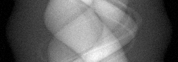
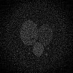
Forward-Model Mismatch Cases
- The widefield fallback produces a spatial image, but MR Spectroscopy acquires frequency-domain spectra encoding chemical composition — metabolite peaks (NAA, choline, creatine, lactate) at specific ppm values are entirely absent
- MRS data is a 1D free induction decay (FID) or spectrum per voxel, not a 2D spatial image — the widefield blur destroys the spectral dimension that encodes metabolite concentrations
How to Correct the Mismatch
- Use the MRS operator that models the free induction decay: y(t) = sum_k(a_k * exp(i*2pi*f_k*t) * exp(-t/T2_k)) for each metabolite k, then FFT to produce the frequency spectrum
- Quantify metabolite concentrations by fitting the spectrum (LCModel, TARQUIN) or using deep-learning spectral quantification with the correctly modeled spectral forward model
Experimental Setup — Signal Chain

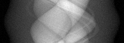
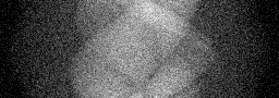
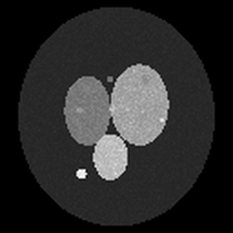
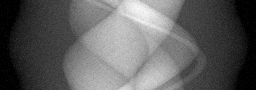
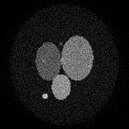
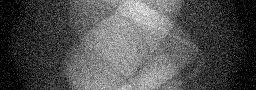
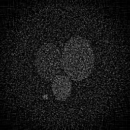
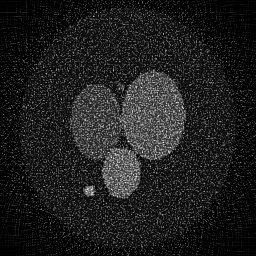
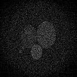
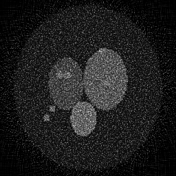
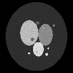
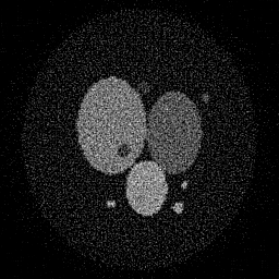
Reconstruction Gallery — 4 Scenes × 3 Scenarios
Method: CPU_baseline | Mismatch: nominal (nominal=True, perturbed=False)

Ground Truth
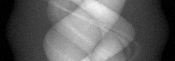
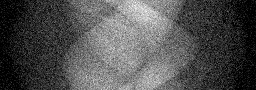
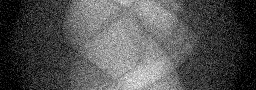
Measurement
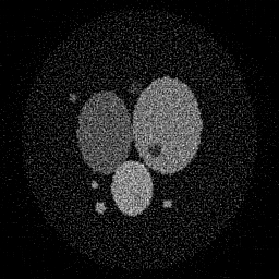
Reconstruction
Ground Truth
Measurement

Reconstruction
Ground Truth
Measurement (perturbed)
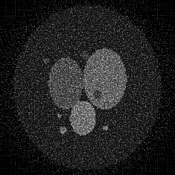
Reconstruction


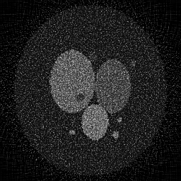
Mean PSNR Across All Scenes
Per-scene PSNR breakdown (4 scenes)
| Scene | I (PSNR) | I (SSIM) | II (PSNR) | II (SSIM) | III (PSNR) | III (SSIM) |
|---|---|---|---|---|---|---|
| scene_00 | 16.584200964385797 | 0.3250905580130585 | 12.506523882319042 | 0.044716474341606735 | 15.931719256055723 | 0.12142227244746187 |
| scene_01 | 18.884299556167566 | 0.3252411352628261 | 13.742128073130111 | 0.048029248758291385 | 17.02391116326154 | 0.11622117666622035 |
| scene_02 | 18.301830801494646 | 0.32976160086547746 | 13.36792873190369 | 0.04964364838717723 | 16.550610792224443 | 0.1259030967011571 |
| scene_03 | 16.67775192548055 | 0.3247822274360334 | 12.53195005733068 | 0.044966709218701925 | 15.850507045662987 | 0.12621817875162467 |
| Mean | 17.61202081188214 | 0.3262188803943489 | 13.037132686170882 | 0.046839020176444326 | 16.33918706430117 | 0.122441181141616 |
Experimental Setup
Key References
- Provencher, 'Estimation of metabolite concentrations from localized in vivo proton NMR spectra (LCModel)', MRM 30, 672-679 (1993)
- Wilson et al., 'Methodological consensus on clinical proton MRS of the brain (MRSinMRS)', NMR in Biomedicine 34, e4484 (2021)
Canonical Datasets
- ISMRM MRS fitting challenge datasets
- Big GABA multi-site MRS data
Spec DAG — Forward Model Pipeline
F(FID) → D(g, η₁)
Mismatch Parameters
| Symbol | Parameter | Description | Nominal | Perturbed |
|---|---|---|---|---|
| Δν | linewidth | Linewidth broadening (Hz) | 0 | 2.0 |
| Δf | freq_drift | Frequency drift (Hz) | 0 | 1.5 |
| Δφ | phase_error | Zero-order phase error (deg) | 0 | 5.0 |
| B | baseline | Baseline distortion amplitude | 0 | 0.05 |
Credits System
Spec Primitives Reference (11 primitives)
Free-space or medium propagation kernel (Fresnel, Rayleigh-Sommerfeld).
Spatial or spatio-temporal amplitude modulation (coded aperture, SLM pattern).
Geometric projection operator (Radon transform, fan-beam, cone-beam).
Sampling in the Fourier / k-space domain (MRI, ptychography).
Shift-invariant convolution with a point-spread function (PSF).
Summation along a physical dimension (spectral, temporal, angular).
Sensor readout with gain g and noise model η (Gaussian, Poisson, mixed).
Patterned illumination (block, Hadamard, random) applied to the scene.
Spectral dispersion element (prism, grating) with shift α and aperture a.
Sample or gantry rotation (CT, electron tomography).
Spectral filter or monochromator selecting a wavelength band.