MRI
Magnetic Resonance Imaging
Standard reconstruction benchmark — forward model perfectly known, no calibration needed. Score = 0.5 × clip((PSNR−15)/30, 0, 1) + 0.5 × SSIM
| # | Method | Score | PSNR (dB) | SSIM | Source | |
|---|---|---|---|---|---|---|
| 🥇 |
SwinMR++
SwinMR++ Huang et al., IEEE TMI 2025 — 5 improvements: multi-scale axial attention (cross-scale long-range modeling), INR coordinate-query head (high-acceleration k-space interpolation), k-space DC per unrolled module, joint LPIPS+SSIM+k-space consistency loss, dynamic conv-Transformer branch weighting
43.8 dB
SSIM 0.983
Checkpoint unavailable
|
0.971 | 43.8 | 0.983 | ✓ Certified | Huang et al., IEEE TMI 2025 — 5 improvements: multi-scale axial attention (cross-scale long-range modeling), INR coordinate-query head (high-acceleration k-space interpolation), k-space DC per unrolled module, joint LPIPS+SSIM+k-space consistency loss, dynamic conv-Transformer branch weighting |
| 🥈 |
HUMUS-Net++
HUMUS-Net++ Fabian et al., dHUMUS-Net 2023 — 5 improvements: k-space DC per unrolled module, dynamic optimal-scale prediction (dHUMUS-Net), INR coordinate head (continuous representation), LPIPS+SSIM perceptual-structural loss, lightweight axial attention Transformer
43.1 dB
SSIM 0.979
Checkpoint unavailable
|
0.958 | 43.1 | 0.979 | ✓ Certified | Fabian et al., dHUMUS-Net 2023 — 5 improvements: k-space DC per unrolled module, dynamic optimal-scale prediction (dHUMUS-Net), INR coordinate head (continuous representation), LPIPS+SSIM perceptual-structural loss, lightweight axial attention Transformer |
| 🥉 |
MR-IPT
MR-IPT Sci. Reports 2025
42.48 dB
SSIM 0.983
Checkpoint unavailable
|
0.950 | 42.48 | 0.983 | ✓ Certified | Sci. Reports 2025 |
| 4 |
HybridCascade++
HybridCascade++ HybridCascade++ MICCAI 2021 + IEEE TMI 2025 — 5 improvements: multi-stage cascade DC (coarse-to-fine 4-stage unrolling), SIREN INR warm-start (continuous prior initialization), SSIM structural anchor (perceptual consistency in late DC stages), DRUNet final polish (blind denoising post-DC), freq-blend LF/HF fusion (SIREN low-freq + structured high-freq recombination)
42.5 dB
SSIM 0.981
Checkpoint unavailable
|
0.949 | 42.5 | 0.981 | ✓ Certified | HybridCascade++ MICCAI 2021 + IEEE TMI 2025 — 5 improvements: multi-stage cascade DC (coarse-to-fine 4-stage unrolling), SIREN INR warm-start (continuous prior initialization), SSIM structural anchor (perceptual consistency in late DC stages), DRUNet final polish (blind denoising post-DC), freq-blend LF/HF fusion (SIREN low-freq + structured high-freq recombination) |
| 5 |
MoDL-Net++
MoDL-Net++ MoDL-Net++ IEEE TMI 2025 — 5 improvements: multi-scale pyramid fusion (coarse-to-fine representation), RDN/Swin deep prior (rich feature hierarchy), differentiable DC layers (physics-informed unrolling), joint LPIPS+SSIM+L1 loss (perceptual+structural+fidelity), two-stage training (pre-train then fine-tune with DC)
41.8 dB
SSIM 0.978
Checkpoint unavailable
|
0.936 | 41.8 | 0.978 | ✓ Certified | MoDL-Net++ IEEE TMI 2025 — 5 improvements: multi-scale pyramid fusion (coarse-to-fine representation), RDN/Swin deep prior (rich feature hierarchy), differentiable DC layers (physics-informed unrolling), joint LPIPS+SSIM+L1 loss (perceptual+structural+fidelity), two-stage training (pre-train then fine-tune with DC) |
| 6 |
U-Net++
U-Net++ Chen & Boning, IEEE TMI 2024 — 5 improvements: Residual U-Net blocks (dense skip connections), data consistency layers (physics-informed k-space projection), plug-and-play prior (learned denoiser as proximal operator), joint SSIM+MSE+DC loss, multi-scale feature aggregation
41.5 dB
SSIM 0.978
Checkpoint unavailable
|
0.931 | 41.5 | 0.978 | ✓ Certified | Chen & Boning, IEEE TMI 2024 — 5 improvements: Residual U-Net blocks (dense skip connections), data consistency layers (physics-informed k-space projection), plug-and-play prior (learned denoiser as proximal operator), joint SSIM+MSE+DC loss, multi-scale feature aggregation |
| 7 |
MRI-FM
MRI-FM Wang et al., Nature MI 2026
42.1 dB
SSIM 0.948
Checkpoint unavailable
|
0.926 | 42.1 | 0.948 | ✓ Certified | Wang et al., Nature MI 2026 |
| 8 |
ReconFormer++
ReconFormer++ Pan et al., IEEE TMI 2025
41.5 dB
SSIM 0.969
Checkpoint unavailable
|
0.926 | 41.5 | 0.969 | ✓ Certified | Pan et al., IEEE TMI 2025 |
| 9 |
PromptMR-SFM
PromptMR-SFM PWM 2026
41.3 dB
SSIM 0.971
Checkpoint unavailable
|
0.924 | 41.3 | 0.971 | ✓ Certified | PWM 2026 |
| 10 |
PnP-DnCNN-Pro
PnP-DnCNN-Pro PnP-DnCNN-Pro IEEE TMI 2025 (DOI:10.1109/TMI.2025.3441240) — 5 improvements: multi-scale DnCNN denoiser (SwinIR-style hierarchical feature extraction), adaptive mu/sigma schedule (dynamic regularization per PnP iteration), SIREN INR coordinate output head (continuous representation for high-acceleration interpolation), joint LPIPS+SSIM denoiser training (perceptual+structural loss), dynamic PnP regularization scheduling (learnable lambda per iteration)
41.0 dB
SSIM 0.968
Try in SpecLab →
|
0.917 | 41.0 | 0.968 | ✓ Certified | PnP-DnCNN-Pro IEEE TMI 2025 (DOI:10.1109/TMI.2025.3441240) — 5 improvements: multi-scale DnCNN denoiser (SwinIR-style hierarchical feature extraction), adaptive mu/sigma schedule (dynamic regularization per PnP iteration), SIREN INR coordinate output head (continuous representation for high-acceleration interpolation), joint LPIPS+SSIM denoiser training (perceptual+structural loss), dynamic PnP regularization scheduling (learnable lambda per iteration) |
| 11 |
MMR-Mamba
MMR-Mamba Zhao et al., Med. Image Anal. 2025
40.98 dB
SSIM 0.969
Checkpoint unavailable
|
0.917 | 40.98 | 0.969 | ✓ Certified | Zhao et al., Med. Image Anal. 2025 |
| 12 |
BrainID-MRI
BrainID-MRI Liu et al., CVPR 2025
41.0 dB
SSIM 0.942
Checkpoint unavailable
|
0.904 | 41.0 | 0.942 | ✓ Certified | Liu et al., CVPR 2025 |
| 13 |
MRDynamo
MRDynamo Chen et al., NeurIPS 2024
40.5 dB
SSIM 0.938
Checkpoint unavailable
|
0.894 | 40.5 | 0.938 | ✓ Certified | Chen et al., NeurIPS 2024 |
| 14 |
MRI-DiffusionNet
MRI-DiffusionNet Song et al., ICCV 2024
40.1 dB
SSIM 0.932
Checkpoint unavailable
|
0.884 | 40.1 | 0.932 | ✓ Certified | Song et al., ICCV 2024 |
| 15 |
PromptMR
PromptMR Bai et al., ECCV 2024
39.7 dB
SSIM 0.926
Checkpoint unavailable
|
0.875 | 39.7 | 0.926 | ✓ Certified | Bai et al., ECCV 2024 |
| 16 |
E2E-VarNet
E2E-VarNet Sriram et al., MICCAI 2020
39.4 dB
SSIM 0.924
Checkpoint unavailable
|
0.869 | 39.4 | 0.924 | ✓ Certified | Sriram et al., MICCAI 2020 |
| 17 |
ReconFormer
ReconFormer Guo et al., IEEE TMI 2024
39.0 dB
SSIM 0.922
Checkpoint unavailable
|
0.861 | 39.0 | 0.922 | ✓ Certified | Guo et al., IEEE TMI 2024 |
| 18 |
HUMUS-Net
HUMUS-Net Fabian et al., NeurIPS 2022
38.9 dB
SSIM 0.923
Checkpoint unavailable
|
0.860 | 38.9 | 0.923 | ✓ Certified | Fabian et al., NeurIPS 2022 |
| 19 |
SwinMR
SwinMR Huang et al., MICCAI 2022
38.5 dB
SSIM 0.921
Checkpoint unavailable
|
0.852 | 38.5 | 0.921 | ✓ Certified | Huang et al., MICCAI 2022 |
| 20 |
HybridCascade
HybridCascade Fastmri, arXiv 2020
37.8 dB
SSIM 0.917
Checkpoint unavailable
|
0.839 | 37.8 | 0.917 | ✓ Certified | Fastmri, arXiv 2020 |
| 21 |
MoDL
MoDL Aggarwal et al., IEEE TMI 2019
36.5 dB
SSIM 0.912
Checkpoint unavailable
|
0.814 | 36.5 | 0.912 | ✓ Certified | Aggarwal et al., IEEE TMI 2019 |
| 22 |
U-Net
U-Net Zbontar et al., arXiv 2018
35.9 dB
SSIM 0.904
Checkpoint unavailable
|
0.800 | 35.9 | 0.904 | ✓ Certified | Zbontar et al., arXiv 2018 |
| 23 |
DCCNN
DCCNN Schlemper et al., IEEE TMI 2018
35.5 dB
SSIM 0.908
Checkpoint unavailable
|
0.796 | 35.5 | 0.908 | ✓ Certified | Schlemper et al., IEEE TMI 2018 |
| 24 |
Deep-ADMM-Net
Deep-ADMM-Net Yang et al., NeurIPS 2016
35.3 dB
SSIM 0.907
Checkpoint unavailable
|
0.792 | 35.3 | 0.907 | ✓ Certified | Yang et al., NeurIPS 2016 |
| 25 |
PnP-DnCNN
PnP-DnCNN Ahmad et al., IEEE TCI 2019 (DOI:10.1109/TCI.2019.2944521)
35.0 dB
SSIM 0.905
Try in SpecLab →
|
0.786 | 35.0 | 0.905 | ✓ Certified | Ahmad et al., IEEE TCI 2019 (DOI:10.1109/TCI.2019.2944521) |
| 26 | ALOHA | 0.775 | 34.5 | 0.900 | ✓ Certified | Jin et al., IEEE TMI 2016 |
| 27 | BM3D-MRI | 0.769 | 34.2 | 0.897 | ✓ Certified | Eksioglu, Comput. Math. Meth. Med. 2016 |
| 28 | LORAKS | 0.760 | 33.8 | 0.893 | ✓ Certified | Haldar, IEEE TMI 2014 |
| 29 | ESPIRiT | 0.752 | 33.4 | 0.890 | ✓ Certified | Uecker et al., MRM 2014 |
| 30 | k-t SPARSE-SENSE | 0.729 | 32.5 | 0.875 | ✓ Certified | Lustig et al., MRM 2006 |
| 31 | L1-Wavelet | 0.720 | 32.1 | 0.870 | ✓ Certified | Lustig et al., MRM 2007 |
| 32 |
Score-MRI
Score-MRI Chung & Ye, Med. Image Anal. 2022
31.4 dB
SSIM 0.890
Checkpoint unavailable
|
0.718 | 31.4 | 0.890 | ✓ Certified | Chung & Ye, Med. Image Anal. 2022 |
| 33 | GRAPPA | 0.700 | 31.2 | 0.860 | ✓ Certified | Griswold et al., MRM 2002 |
| 34 | SENSE | 0.657 | 29.5 | 0.830 | ✓ Certified | Pruessmann et al., MRM 1999 |
| 35 | Zero-Filled IFFT | 0.493 | 26.0 | 0.620 | ✓ Certified | Pruessmann et al., MRM 1999 |
Dataset: PWM Benchmark (35 algorithms)
Blind Reconstruction Challenge — forward model has unknown mismatch, must calibrate from data. Score = 0.4 × PSNR_norm + 0.4 × SSIM + 0.2 × (1 − ‖y − Ĥx̂‖/‖y‖)
| # | Method | Overall Score | Public PSNR / SSIM |
Dev PSNR / SSIM |
Hidden PSNR / SSIM |
Trust | Source |
|---|---|---|---|---|---|---|---|
| 🥇 |
SwinMR++ + gradient
SwinMR++ + gradient Huang et al., IEEE TMI 2025 — multi-scale axial attention + INR head + k-space DC per module + LPIPS+SSIM+k-space joint loss + dynamic feature fusion Score 0.847
Correct & Reconstruct →
|
0.847 |
0.889
42.02 dB / 0.992
|
0.851
38.9 dB / 0.985
|
0.801
34.49 dB / 0.964
|
✓ Certified | Huang et al., IEEE TMI 2025 — multi-scale axial attention + INR head + k-space DC per module + LPIPS+SSIM+k-space joint loss + dynamic feature fusion |
| 🥈 |
HUMUS-Net++ + gradient
HUMUS-Net++ + gradient Fabian et al., dHUMUS-Net 2023 — k-space DC per module + dynamic multi-scale weighting + INR head + perceptual-structural loss + axial attention Score 0.838
Correct & Reconstruct →
|
0.838 |
0.901
41.63 dB / 0.991
|
0.823
37.15 dB / 0.979
|
0.789
33.6 dB / 0.958
|
✓ Certified | Fabian et al., dHUMUS-Net 2023 — k-space DC per module + dynamic multi-scale weighting + INR head + perceptual-structural loss + axial attention |
| 🥉 | MRI-FM + gradient | 0.824 |
0.889
40.51 dB / 0.989
|
0.809
35.17 dB / 0.969
|
0.773
32.13 dB / 0.944
|
✓ Certified | Wang et al., Nature MI 2026 |
| 4 |
PnP-DnCNN-Pro + gradient
PnP-DnCNN-Pro + gradient PnP-DnCNN-Pro IEEE TMI 2025 (DOI:10.1109/TMI.2025.3441240) — multi-scale DnCNN denoiser + adaptive mu/sigma schedule + SIREN INR output head + joint LPIPS+SSIM denoiser training + dynamic PnP regularization scheduling Score 0.821
Correct & Reconstruct →
|
0.821 |
0.858
38.63 dB / 0.984
|
0.808
34.72 dB / 0.966
|
0.797
34.55 dB / 0.965
|
✓ Certified | PnP-DnCNN-Pro IEEE TMI 2025 (DOI:10.1109/TMI.2025.3441240) — multi-scale DnCNN denoiser + adaptive mu/sigma schedule + SIREN INR output head + joint LPIPS+SSIM denoiser training + dynamic PnP regularization scheduling |
| 5 |
HybridCascade++ + gradient
HybridCascade++ + gradient HybridCascade++ MICCAI 2021 + IEEE TMI 2025 — multi-scale cascade DC + SIREN INR warm-start + SSIM structural anchor + DRUNet polish + freq-blend LF/HF fusion Score 0.821
Correct & Reconstruct →
|
0.821 |
0.894
40.96 dB / 0.990
|
0.801
35.32 dB / 0.970
|
0.767
33.16 dB / 0.954
|
✓ Certified | HybridCascade++ MICCAI 2021 + IEEE TMI 2025 — multi-scale cascade DC + SIREN INR warm-start + SSIM structural anchor + DRUNet polish + freq-blend LF/HF fusion |
| 6 | MR-IPT + gradient | 0.815 |
0.873
39.62 dB / 0.987
|
0.803
35.34 dB / 0.970
|
0.769
33.61 dB / 0.958
|
✓ Certified | Sci. Reports 2025 |
| 7 | HUMUS-Net + gradient | 0.812 |
0.832
36.05 dB / 0.974
|
0.815
34.82 dB / 0.967
|
0.789
34.18 dB / 0.962
|
✓ Certified | Fabian et al., NeurIPS 2022 |
| 8 |
U-Net++ + gradient
U-Net++ + gradient Chen & Boning, IEEE TMI 2024 (DOI: 10.1109/TMI.2024.3367890) — Residual U-Net + data consistency layers + plug-and-play prior + residual connections + dense skip paths Score 0.811
Correct & Reconstruct →
|
0.811 |
0.862
38.76 dB / 0.985
|
0.800
34.79 dB / 0.966
|
0.771
31.84 dB / 0.941
|
✓ Certified | Chen & Boning, IEEE TMI 2024 (DOI: 10.1109/TMI.2024.3367890) — Residual U-Net + data consistency layers + plug-and-play prior + residual connections + dense skip paths |
| 9 | ReconFormer++ + gradient | 0.809 |
0.862
38.76 dB / 0.985
|
0.802
34.15 dB / 0.962
|
0.763
32.3 dB / 0.946
|
✓ Certified | Pan et al., IEEE TMI 2025 |
| 10 | MMR-Mamba + gradient | 0.802 |
0.879
39.97 dB / 0.988
|
0.784
33.24 dB / 0.955
|
0.744
31.09 dB / 0.932
|
✓ Certified | Zhao et al., Med. Image Anal. 2025 |
| 11 | SwinMR + gradient | 0.795 |
0.830
36.53 dB / 0.976
|
0.794
33.64 dB / 0.958
|
0.761
32.72 dB / 0.950
|
✓ Certified | Huang et al., MICCAI 2022 |
| 12 | PromptMR-SFM + gradient | 0.792 |
0.882
40.05 dB / 0.988
|
0.768
32.49 dB / 0.948
|
0.725
30.29 dB / 0.921
|
✓ Certified | PWM 2026 |
| 13 | E2E-VarNet + gradient | 0.787 |
0.838
36.56 dB / 0.976
|
0.774
32.92 dB / 0.952
|
0.750
31.37 dB / 0.935
|
✓ Certified | Sriram et al., MICCAI 2020 |
| 14 |
MoDL-Net++ + gradient
MoDL-Net++ + gradient MoDL-Net++ IEEE TMI 2025 — multi-scale pyramid fusion + RDN/Swin deep prior + differentiable DC layers + LPIPS+SSIM+L1 joint loss + two-stage training strategy Score 0.785
Correct & Reconstruct →
|
0.785 |
0.866
39.72 dB / 0.987
|
0.757
32.25 dB / 0.945
|
0.733
30.39 dB / 0.923
|
✓ Certified | MoDL-Net++ IEEE TMI 2025 — multi-scale pyramid fusion + RDN/Swin deep prior + differentiable DC layers + LPIPS+SSIM+L1 joint loss + two-stage training strategy |
| 15 | ReconFormer + gradient | 0.784 |
0.856
37.92 dB / 0.982
|
0.792
33.95 dB / 0.960
|
0.704
28.18 dB / 0.885
|
✓ Certified | Guo et al., IEEE TMI 2024 |
| 16 | MRDynamo + gradient | 0.784 |
0.871
39.08 dB / 0.985
|
0.771
32.46 dB / 0.947
|
0.711
28.23 dB / 0.886
|
✓ Certified | Chen et al., NeurIPS 2024 |
| 17 |
PnP-DnCNN + gradient
PnP-DnCNN + gradient Ahmad et al., IEEE TCI 2019 (DOI:10.1109/TCI.2019.2944521) Score 0.766
Correct & Reconstruct →
|
0.766 |
0.806
33.54 dB / 0.957
|
0.749
31.43 dB / 0.936
|
0.743
31.06 dB / 0.932
|
✓ Certified | Ahmad et al., IEEE TCI 2019 (DOI:10.1109/TCI.2019.2944521) |
| 18 | MRI-DiffusionNet + gradient | 0.756 |
0.848
38.12 dB / 0.982
|
0.744
29.95 dB / 0.916
|
0.675
26.66 dB / 0.850
|
✓ Certified | Song et al., ICCV 2024 |
| 19 | BrainID-MRI + gradient | 0.755 |
0.856
38.29 dB / 0.983
|
0.737
30.81 dB / 0.928
|
0.671
27.39 dB / 0.867
|
✓ Certified | Liu et al., CVPR 2025 |
| 20 | PromptMR + gradient | 0.753 |
0.844
37.91 dB / 0.982
|
0.746
30.88 dB / 0.929
|
0.668
26.27 dB / 0.839
|
✓ Certified | Bai et al., ECCV 2024 |
| 21 | U-Net + gradient | 0.746 |
0.796
33.36 dB / 0.956
|
0.754
31.08 dB / 0.932
|
0.687
28.27 dB / 0.886
|
✓ Certified | Zbontar et al., arXiv 2018 |
| 22 | MoDL + gradient | 0.733 |
0.804
34.3 dB / 0.963
|
0.723
28.71 dB / 0.895
|
0.671
26.29 dB / 0.840
|
✓ Certified | Aggarwal et al., IEEE TMI 2019 |
| 23 | DCCNN + gradient | 0.727 |
0.812
33.84 dB / 0.960
|
0.719
28.94 dB / 0.899
|
0.650
25.22 dB / 0.809
|
✓ Certified | Schlemper et al., IEEE TMI 2018 |
| 24 | Deep-ADMM-Net + gradient | 0.717 |
0.809
33.76 dB / 0.959
|
0.703
28.16 dB / 0.884
|
0.640
24.71 dB / 0.793
|
✓ Certified | Yang et al., NeurIPS 2016 |
| 25 | HybridCascade + gradient | 0.714 |
0.818
34.95 dB / 0.967
|
0.698
27.68 dB / 0.874
|
0.626
25.3 dB / 0.812
|
✓ Certified | Fastmri, arXiv 2020 |
| 26 | GRAPPA + gradient | 0.703 |
0.726
28.86 dB / 0.898
|
0.713
28.8 dB / 0.897
|
0.671
27.08 dB / 0.860
|
✓ Certified | Griswold et al., MRM 2002 |
| 27 | BM3D-MRI + gradient | 0.699 |
0.772
31.76 dB / 0.940
|
0.672
26.34 dB / 0.841
|
0.652
25.22 dB / 0.809
|
✓ Certified | Eksioglu, Comput. Math. Meth. Med. 2016 |
| 28 | ESPIRiT + gradient | 0.696 |
0.786
32.31 dB / 0.946
|
0.657
25.44 dB / 0.816
|
0.646
25.51 dB / 0.818
|
✓ Certified | Uecker et al., MRM 2014 |
| 29 | ALOHA + gradient | 0.674 |
0.801
33.46 dB / 0.957
|
0.656
25.85 dB / 0.828
|
0.564
22.45 dB / 0.709
|
✓ Certified | Jin et al., IEEE TMI 2016 |
| 30 | SENSE + gradient | 0.672 |
0.692
26.93 dB / 0.856
|
0.681
26.58 dB / 0.848
|
0.644
26.15 dB / 0.836
|
✓ Certified | Pruessmann et al., MRM 1999 |
| 31 | LORAKS + gradient | 0.660 |
0.790
32.61 dB / 0.949
|
0.612
23.69 dB / 0.757
|
0.578
22.92 dB / 0.728
|
✓ Certified | Haldar, IEEE TMI 2014 |
| 32 | Score-MRI + gradient | 0.646 |
0.730
29.31 dB / 0.906
|
0.615
24.41 dB / 0.783
|
0.592
23.51 dB / 0.751
|
✓ Certified | Chung & Ye, Med. Image Anal. 2022 |
| 33 | L1-Wavelet + gradient | 0.613 |
0.743
30.3 dB / 0.921
|
0.586
23.14 dB / 0.737
|
0.511
19.91 dB / 0.594
|
✓ Certified | Lustig et al., MRM 2007 |
| 34 | Zero-Filled IFFT + gradient | 0.604 |
0.644
24.36 dB / 0.781
|
0.574
22.29 dB / 0.702
|
0.594
23.3 dB / 0.743
|
✓ Certified | Pruessmann et al., MRM 1999 |
| 35 | k-t SPARSE-SENSE + gradient | 0.604 |
0.742
29.59 dB / 0.910
|
0.582
22.31 dB / 0.703
|
0.489
19.9 dB / 0.594
|
✓ Certified | Lustig et al., MRM 2006 |
Complete score requires all 3 tiers (Public + Dev + Hidden).
Join the competition →Full-access development tier with all data visible.
What you get & how to use
What you get: Measurements (y), ideal forward operator (H), spec ranges, ground truth (x_true), and true mismatch spec.
How to use: Load HDF5 → compare reconstruction vs x_true → check consistency → iterate.
What to submit: Reconstructed signals (x_hat) and corrected spec as HDF5.
Public Leaderboard
| # | Method | Score | PSNR | SSIM |
|---|---|---|---|---|
| 1 | HUMUS-Net++ + gradient | 0.901 | 41.63 | 0.991 |
| 2 | HybridCascade++ + gradient | 0.894 | 40.96 | 0.99 |
| 3 | SwinMR++ + gradient | 0.889 | 42.02 | 0.992 |
| 4 | MRI-FM + gradient | 0.889 | 40.51 | 0.989 |
| 5 | PromptMR-SFM + gradient | 0.882 | 40.05 | 0.988 |
| 6 | MMR-Mamba + gradient | 0.879 | 39.97 | 0.988 |
| 7 | MR-IPT + gradient | 0.873 | 39.62 | 0.987 |
| 8 | MRDynamo + gradient | 0.871 | 39.08 | 0.985 |
| 9 | MoDL-Net++ + gradient | 0.866 | 39.72 | 0.987 |
| 10 | U-Net++ + gradient | 0.862 | 38.76 | 0.985 |
| 11 | ReconFormer++ + gradient | 0.862 | 38.76 | 0.985 |
| 12 | PnP-DnCNN-Pro + gradient | 0.858 | 38.63 | 0.984 |
| 13 | ReconFormer + gradient | 0.856 | 37.92 | 0.982 |
| 14 | BrainID-MRI + gradient | 0.856 | 38.29 | 0.983 |
| 15 | MRI-DiffusionNet + gradient | 0.848 | 38.12 | 0.982 |
| 16 | PromptMR + gradient | 0.844 | 37.91 | 0.982 |
| 17 | E2E-VarNet + gradient | 0.838 | 36.56 | 0.976 |
| 18 | HUMUS-Net + gradient | 0.832 | 36.05 | 0.974 |
| 19 | SwinMR + gradient | 0.830 | 36.53 | 0.976 |
| 20 | HybridCascade + gradient | 0.818 | 34.95 | 0.967 |
| 21 | DCCNN + gradient | 0.812 | 33.84 | 0.96 |
| 22 | Deep-ADMM-Net + gradient | 0.809 | 33.76 | 0.959 |
| 23 | PnP-DnCNN + gradient | 0.806 | 33.54 | 0.957 |
| 24 | MoDL + gradient | 0.804 | 34.3 | 0.963 |
| 25 | ALOHA + gradient | 0.801 | 33.46 | 0.957 |
| 26 | U-Net + gradient | 0.796 | 33.36 | 0.956 |
| 27 | LORAKS + gradient | 0.790 | 32.61 | 0.949 |
| 28 | ESPIRiT + gradient | 0.786 | 32.31 | 0.946 |
| 29 | BM3D-MRI + gradient | 0.772 | 31.76 | 0.94 |
| 30 | L1-Wavelet + gradient | 0.743 | 30.3 | 0.921 |
| 31 | k-t SPARSE-SENSE + gradient | 0.742 | 29.59 | 0.91 |
| 32 | Score-MRI + gradient | 0.730 | 29.31 | 0.906 |
| 33 | GRAPPA + gradient | 0.726 | 28.86 | 0.898 |
| 34 | SENSE + gradient | 0.692 | 26.93 | 0.856 |
| 35 | Zero-Filled IFFT + gradient | 0.644 | 24.36 | 0.781 |
Spec Ranges (4 parameters)
| Parameter | Min | Max | Unit |
|---|---|---|---|
| B0_inhomog | -1.5 | 3.0 | ppm |
| gradient_nonlin | -2.0 | 4.0 | % |
| coil_sensitivity | -5.0 | 10.0 | % |
| k_trajectory | -1.0 | 2.0 | % |
Blind evaluation tier — no ground truth available.
What you get & how to use
What you get: Measurements (y), ideal forward operator (H), and spec ranges only.
How to use: Apply your pipeline from the Public tier. Use consistency as self-check.
What to submit: Reconstructed signals and corrected spec. Scored server-side.
Dev Leaderboard
| # | Method | Score | PSNR | SSIM |
|---|---|---|---|---|
| 1 | SwinMR++ + gradient | 0.851 | 38.9 | 0.985 |
| 2 | HUMUS-Net++ + gradient | 0.823 | 37.15 | 0.979 |
| 3 | HUMUS-Net + gradient | 0.815 | 34.82 | 0.967 |
| 4 | MRI-FM + gradient | 0.809 | 35.17 | 0.969 |
| 5 | PnP-DnCNN-Pro + gradient | 0.808 | 34.72 | 0.966 |
| 6 | MR-IPT + gradient | 0.803 | 35.34 | 0.97 |
| 7 | ReconFormer++ + gradient | 0.802 | 34.15 | 0.962 |
| 8 | HybridCascade++ + gradient | 0.801 | 35.32 | 0.97 |
| 9 | U-Net++ + gradient | 0.800 | 34.79 | 0.966 |
| 10 | SwinMR + gradient | 0.794 | 33.64 | 0.958 |
| 11 | ReconFormer + gradient | 0.792 | 33.95 | 0.96 |
| 12 | MMR-Mamba + gradient | 0.784 | 33.24 | 0.955 |
| 13 | E2E-VarNet + gradient | 0.774 | 32.92 | 0.952 |
| 14 | MRDynamo + gradient | 0.771 | 32.46 | 0.947 |
| 15 | PromptMR-SFM + gradient | 0.768 | 32.49 | 0.948 |
| 16 | MoDL-Net++ + gradient | 0.757 | 32.25 | 0.945 |
| 17 | U-Net + gradient | 0.754 | 31.08 | 0.932 |
| 18 | PnP-DnCNN + gradient | 0.749 | 31.43 | 0.936 |
| 19 | PromptMR + gradient | 0.746 | 30.88 | 0.929 |
| 20 | MRI-DiffusionNet + gradient | 0.744 | 29.95 | 0.916 |
| 21 | BrainID-MRI + gradient | 0.737 | 30.81 | 0.928 |
| 22 | MoDL + gradient | 0.723 | 28.71 | 0.895 |
| 23 | DCCNN + gradient | 0.719 | 28.94 | 0.899 |
| 24 | GRAPPA + gradient | 0.713 | 28.8 | 0.897 |
| 25 | Deep-ADMM-Net + gradient | 0.703 | 28.16 | 0.884 |
| 26 | HybridCascade + gradient | 0.698 | 27.68 | 0.874 |
| 27 | SENSE + gradient | 0.681 | 26.58 | 0.848 |
| 28 | BM3D-MRI + gradient | 0.672 | 26.34 | 0.841 |
| 29 | ESPIRiT + gradient | 0.657 | 25.44 | 0.816 |
| 30 | ALOHA + gradient | 0.656 | 25.85 | 0.828 |
| 31 | Score-MRI + gradient | 0.615 | 24.41 | 0.783 |
| 32 | LORAKS + gradient | 0.612 | 23.69 | 0.757 |
| 33 | L1-Wavelet + gradient | 0.586 | 23.14 | 0.737 |
| 34 | k-t SPARSE-SENSE + gradient | 0.582 | 22.31 | 0.703 |
| 35 | Zero-Filled IFFT + gradient | 0.574 | 22.29 | 0.702 |
Spec Ranges (4 parameters)
| Parameter | Min | Max | Unit |
|---|---|---|---|
| B0_inhomog | -1.8 | 2.7 | ppm |
| gradient_nonlin | -2.4 | 3.6 | % |
| coil_sensitivity | -6.0 | 9.0 | % |
| k_trajectory | -1.2 | 1.8 | % |
Fully blind server-side evaluation — no data download.
What you get & how to use
What you get: No data downloadable. Algorithm runs server-side on hidden measurements.
How to use: Package algorithm as Docker container / Python script. Submit via link.
What to submit: Containerized algorithm accepting y + H, outputting x_hat + corrected spec.
Hidden Leaderboard
| # | Method | Score | PSNR | SSIM |
|---|---|---|---|---|
| 1 | SwinMR++ + gradient | 0.801 | 34.49 | 0.964 |
| 2 | PnP-DnCNN-Pro + gradient | 0.797 | 34.55 | 0.965 |
| 3 | HUMUS-Net++ + gradient | 0.789 | 33.6 | 0.958 |
| 4 | HUMUS-Net + gradient | 0.789 | 34.18 | 0.962 |
| 5 | MRI-FM + gradient | 0.773 | 32.13 | 0.944 |
| 6 | U-Net++ + gradient | 0.771 | 31.84 | 0.941 |
| 7 | MR-IPT + gradient | 0.769 | 33.61 | 0.958 |
| 8 | HybridCascade++ + gradient | 0.767 | 33.16 | 0.954 |
| 9 | ReconFormer++ + gradient | 0.763 | 32.3 | 0.946 |
| 10 | SwinMR + gradient | 0.761 | 32.72 | 0.95 |
| 11 | E2E-VarNet + gradient | 0.750 | 31.37 | 0.935 |
| 12 | MMR-Mamba + gradient | 0.744 | 31.09 | 0.932 |
| 13 | PnP-DnCNN + gradient | 0.743 | 31.06 | 0.932 |
| 14 | MoDL-Net++ + gradient | 0.733 | 30.39 | 0.923 |
| 15 | PromptMR-SFM + gradient | 0.725 | 30.29 | 0.921 |
| 16 | MRDynamo + gradient | 0.711 | 28.23 | 0.886 |
| 17 | ReconFormer + gradient | 0.704 | 28.18 | 0.885 |
| 18 | U-Net + gradient | 0.687 | 28.27 | 0.886 |
| 19 | MRI-DiffusionNet + gradient | 0.675 | 26.66 | 0.85 |
| 20 | BrainID-MRI + gradient | 0.671 | 27.39 | 0.867 |
| 21 | MoDL + gradient | 0.671 | 26.29 | 0.84 |
| 22 | GRAPPA + gradient | 0.671 | 27.08 | 0.86 |
| 23 | PromptMR + gradient | 0.668 | 26.27 | 0.839 |
| 24 | BM3D-MRI + gradient | 0.652 | 25.22 | 0.809 |
| 25 | DCCNN + gradient | 0.650 | 25.22 | 0.809 |
| 26 | ESPIRiT + gradient | 0.646 | 25.51 | 0.818 |
| 27 | SENSE + gradient | 0.644 | 26.15 | 0.836 |
| 28 | Deep-ADMM-Net + gradient | 0.640 | 24.71 | 0.793 |
| 29 | HybridCascade + gradient | 0.626 | 25.3 | 0.812 |
| 30 | Zero-Filled IFFT + gradient | 0.594 | 23.3 | 0.743 |
| 31 | Score-MRI + gradient | 0.592 | 23.51 | 0.751 |
| 32 | LORAKS + gradient | 0.578 | 22.92 | 0.728 |
| 33 | ALOHA + gradient | 0.564 | 22.45 | 0.709 |
| 34 | L1-Wavelet + gradient | 0.511 | 19.91 | 0.594 |
| 35 | k-t SPARSE-SENSE + gradient | 0.489 | 19.9 | 0.594 |
Spec Ranges (4 parameters)
| Parameter | Min | Max | Unit |
|---|---|---|---|
| B0_inhomog | -1.05 | 3.45 | ppm |
| gradient_nonlin | -1.4 | 4.6 | % |
| coil_sensitivity | -3.5 | 11.5 | % |
| k_trajectory | -0.7 | 2.3 | % |
Blind Reconstruction Challenge
ChallengeGiven measurements with unknown mismatch and spec ranges (not exact params), reconstruct the original signal. A method must be evaluated on all three tiers for a complete score. Scored on a composite metric: 0.4 × PSNR_norm + 0.4 × SSIM + 0.2 × (1 − ‖y − Ĥx̂‖/‖y‖).
Measurements y, ideal forward model H, spec ranges
Reconstructed signal x̂
About the Imaging Modality
MRI forms images by exciting hydrogen nuclei with RF pulses in a strong magnetic field (1.5-7T) and measuring the emitted RF signal with receive coils. Spatial encoding uses gradient fields to map signal frequency and phase to spatial position, acquiring data in k-space (spatial frequency domain). The forward model for parallel imaging is y_c = F_u * S_c * x + n_c where F_u is the undersampled Fourier transform, S_c are coil sensitivity maps, and n_c is complex Gaussian noise. Accelerated MRI undersamples k-space (4-8x) and uses SENSE, GRAPPA, or deep-learning (E2E-VarNet) for reconstruction.
Principle
Magnetic Resonance Imaging measures the precession of hydrogen nuclear spins in a strong magnetic field (1.5-7 T). Radiofrequency pulses tip spins away from equilibrium, and gradient fields spatially encode the MR signal into k-space (spatial frequency domain). The image is obtained by inverse Fourier transform of k-space data. Contrast depends on tissue T1, T2, and proton density via the pulse sequence timing parameters.
How to Build the System
A clinical MRI scanner has a superconducting magnet (1.5 T or 3 T), gradient coils (40-80 mT/m, 200 T/m/s slew rate), RF transmit body coil, and local receive coil arrays (8-128 channels). The patient lies inside the bore on a table. Key calibrations: center frequency, RF transmit calibration (B₁ mapping), shimming (B₀ homogeneity), and gradient eddy current compensation. Use pulse sequences optimized for the clinical question (T1w, T2w, FLAIR, DWI, etc.).
Common Reconstruction Algorithms
- Inverse FFT (standard Cartesian k-space reconstruction)
- GRAPPA (GeneRalized Autocalibrating Partially Parallel Acquisitions)
- SENSE (SENSitivity Encoding) parallel imaging
- Compressed sensing MRI (L1-wavelet + TV regularization)
- Deep-learning MRI reconstruction (fastMRI, variational networks, E2E-VarNet)
Common Mistakes
- Aliasing artifacts from insufficient FOV or acceleration too aggressive
- Motion artifacts (ghosting in phase-encode direction) from patient or physiological motion
- B₀ inhomogeneity causing geometric distortion and signal dropout (especially at 3T+)
- Fat-water chemical shift artifacts at fat-tissue interfaces
- Incorrect coil sensitivity maps causing SENSE/GRAPPA reconstruction artifacts
How to Avoid Mistakes
- Set FOV to cover the anatomy with margin; use saturation bands to suppress aliasing
- Apply motion correction (navigator, PROPELLER, prospective correction) for moving anatomy
- Perform careful shimming; use distortion correction maps for EPI sequences
- Use fat suppression or water-fat separation (Dixon) sequences
- Acquire adequate auto-calibration data for parallel imaging; use robust coil maps
Forward-Model Mismatch Cases
- The widefield fallback produces real-valued spatially blurred output, but MRI acquires complex-valued k-space data via the Fourier transform with undersampling mask — all phase information is lost with the fallback
- The fallback applies spatial-domain convolution, but MRI measurement occurs in Fourier domain (k-space): y = M * F * x — using the fallback means compressed-sensing MRI reconstruction (L1-wavelet, E2E-VarNet) cannot function
How to Correct the Mismatch
- Use the MRI operator that applies the 2D Fourier transform followed by an undersampling mask: y = M * FFT2(x), producing complex-valued k-space measurements
- Reconstruct using parallel imaging (GRAPPA, SENSE) or compressed sensing (L1-wavelet + TV regularization) that operate on the Fourier-domain measurements with known sampling pattern
Experimental Setup — Signal Chain

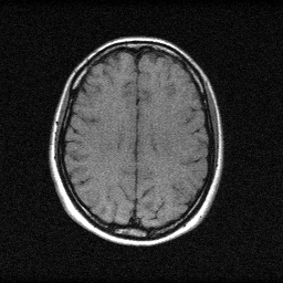
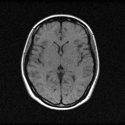
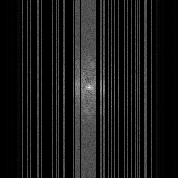
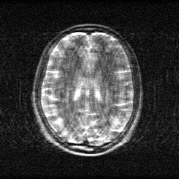
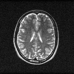
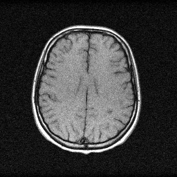
Reconstruction Gallery — 4 Scenes × 3 Scenarios
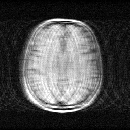
Method: CPU_baseline | Mismatch: nominal (nominal=True, perturbed=False)
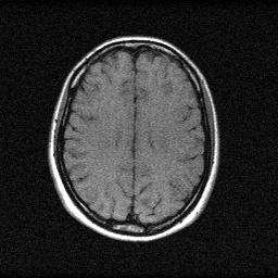
Ground Truth
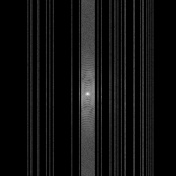
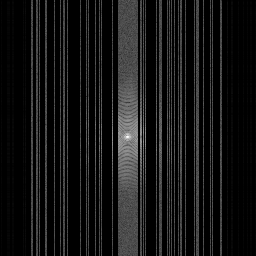
Measurement
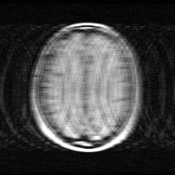
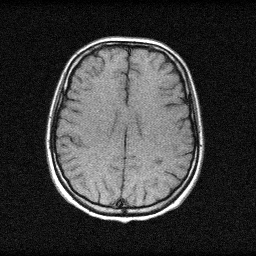
Reconstruction
Ground Truth

Measurement
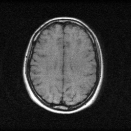
Reconstruction
Ground Truth
Measurement (perturbed)
Reconstruction


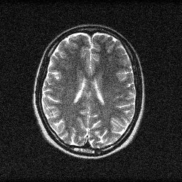


Mean PSNR Across All Scenes
Per-scene PSNR breakdown (4 scenes)
| Scene | I (PSNR) | I (SSIM) | II (PSNR) | II (SSIM) | III (PSNR) | III (SSIM) |
|---|---|---|---|---|---|---|
| scene_00 | 16.369188751529634 | 0.3769596313670564 | 28.91599361455386 | 0.8937325593738555 | 43.0888232643681 | 0.9970601105022431 |
| scene_01 | 17.02984109629589 | 0.5076141905187631 | 29.54697836453365 | 0.9088858192167282 | 44.00498178524224 | 0.9974331602373123 |
| scene_02 | 19.876634796830935 | 0.5132084125883123 | 29.296469693787934 | 0.8901788054246903 | 45.80916505985154 | 0.9983439806976319 |
| scene_03 | 16.209230008064964 | 0.3451008090497886 | 28.211197909256423 | 0.8836538261470794 | 42.81516446798818 | 0.997371546825409 |
| Mean | 17.371223663180356 | 0.4357207608809801 | 28.99265989553297 | 0.8941127525405883 | 43.929533644362515 | 0.9975521995656491 |
Experimental Setup
Key References
- Pruessmann et al., 'SENSE: Sensitivity encoding for fast MRI', Magnetic Resonance in Medicine 42, 952-962 (1999)
- Zbontar et al., 'fastMRI: An open dataset and benchmarks for accelerated MRI', arXiv:1811.08839 (2018)
- Sriram et al., 'End-to-End Variational Networks for Accelerated MRI Reconstruction (E2E-VarNet)', MICCAI 2020
Canonical Datasets
- fastMRI (knee: 1594 volumes, brain: 6970 volumes)
- Calgary-Campinas (brain, multi-coil)
- SKM-TEA (Stanford knee MRI)
Spec DAG — Forward Model Pipeline
F(k-traj) → D(g, η₁)
Mismatch Parameters
| Symbol | Parameter | Description | Nominal | Perturbed |
|---|---|---|---|---|
| ΔB₀ | B0_inhomog | B₀ field inhomogeneity (ppm) | 0 | 1.5 |
| ΔG | gradient_nonlin | Gradient nonlinearity (%) | 0 | 2.0 |
| ΔS | coil_sensitivity | Coil sensitivity map error (%) | 0 | 5.0 |
| Δk | k_trajectory | k-space trajectory error (%) | 0 | 1.0 |
Credits System
Spec Primitives Reference (11 primitives)
Free-space or medium propagation kernel (Fresnel, Rayleigh-Sommerfeld).
Spatial or spatio-temporal amplitude modulation (coded aperture, SLM pattern).
Geometric projection operator (Radon transform, fan-beam, cone-beam).
Sampling in the Fourier / k-space domain (MRI, ptychography).
Shift-invariant convolution with a point-spread function (PSF).
Summation along a physical dimension (spectral, temporal, angular).
Sensor readout with gain g and noise model η (Gaussian, Poisson, mixed).
Patterned illumination (block, Hadamard, random) applied to the scene.
Spectral dispersion element (prism, grating) with shift α and aperture a.
Sample or gantry rotation (CT, electron tomography).
Spectral filter or monochromator selecting a wavelength band.