Matrix
Generic Matrix Sensing
Standard reconstruction benchmark — forward model perfectly known, no calibration needed. Score = 0.5 × clip((PSNR−15)/30, 0, 1) + 0.5 × SSIM
| # | Method | Score | PSNR (dB) | SSIM | Source | |
|---|---|---|---|---|---|---|
| 🥇 | FlowHSI | 0.884 | 38.58 | 0.982 | ✓ Certified | Huang et al., arXiv 2025 |
| 🥈 |
ScoreSCI
ScoreSCI Chen et al., NeurIPS 2024
38.22 dB
SSIM 0.980
Checkpoint unavailable
|
0.877 | 38.22 | 0.980 | ✓ Certified | Chen et al., NeurIPS 2024 |
| 🥉 |
DiffusionHSI
DiffusionHSI Zhang et al., ICCV 2024
37.95 dB
SSIM 0.978
Checkpoint unavailable
|
0.872 | 37.95 | 0.978 | ✓ Certified | Zhang et al., ICCV 2024 |
| 4 |
PromptSCI
PromptSCI Bai et al., ICCV 2024
37.35 dB
SSIM 0.975
Checkpoint unavailable
|
0.860 | 37.35 | 0.975 | ✓ Certified | Bai et al., ICCV 2024 |
| 5 |
CSTrans
CSTrans Liu et al., CVPR 2024
37.12 dB
SSIM 0.973
Checkpoint unavailable
|
0.855 | 37.12 | 0.973 | ✓ Certified | Liu et al., CVPR 2024 |
| 6 |
HiSViT+
HiSViT+ Tao et al., ECCV 2024
36.85 dB
SSIM 0.971
Checkpoint unavailable
|
0.850 | 36.85 | 0.971 | ✓ Certified | Tao et al., ECCV 2024 |
| 7 |
CST
CST Liu et al., ICCV 2023
35.92 dB
SSIM 0.965
Checkpoint unavailable
|
0.831 | 35.92 | 0.965 | ✓ Certified | Liu et al., ICCV 2023 |
| 8 |
Restormer
Restormer Zamir et al., CVPR 2022
35.68 dB
SSIM 0.962
Checkpoint unavailable
|
0.826 | 35.68 | 0.962 | ✓ Certified | Zamir et al., CVPR 2022 |
| 9 |
MST-L
MST-L Cai et al., CVPR 2022
35.4 dB
SSIM 0.960
Checkpoint unavailable
|
0.820 | 35.4 | 0.960 | ✓ Certified | Cai et al., CVPR 2022 |
| 10 |
EfficientSCI
EfficientSCI Wang et al., IEEE TIP 2023
34.21 dB
SSIM 0.949
Checkpoint unavailable
|
0.795 | 34.21 | 0.949 | ✓ Certified | Wang et al., IEEE TIP 2023 |
| 11 | PnP-FFDNet | 0.670 | 29.65 | 0.852 | ✓ Certified | Zhang et al., 2017 |
| 12 | TVAL3 | 0.658 | 29.15 | 0.845 | ✓ Certified | Li et al., 2009 |
| 13 | FISTA-TV | 0.634 | 28.42 | 0.821 | ✓ Certified | Beck & Teboulle, 2009 |
| 14 | GAP-TV | 0.574 | 26.83 | 0.754 | ✓ Certified | Yuan et al., 2016 |
Dataset: PWM Benchmark (14 algorithms)
Blind Reconstruction Challenge — forward model has unknown mismatch, must calibrate from data. Score = 0.4 × PSNR_norm + 0.4 × SSIM + 0.2 × (1 − ‖y − Ĥx̂‖/‖y‖)
| # | Method | Overall Score | Public PSNR / SSIM |
Dev PSNR / SSIM |
Hidden PSNR / SSIM |
Trust | Source |
|---|---|---|---|---|---|---|---|
| 🥇 | ScoreSCI + gradient | 0.769 |
0.823
35.47 dB / 0.971
|
0.751
30.77 dB / 0.928
|
0.732
30.43 dB / 0.923
|
✓ Certified | Chen et al., NeurIPS 2024 |
| 🥈 | FlowHSI + gradient | 0.763 |
0.851
37.3 dB / 0.979
|
0.745
30.29 dB / 0.921
|
0.694
28.56 dB / 0.892
|
✓ Certified | Huang et al., arXiv 2025 |
| 🥉 | CSTrans + gradient | 0.754 |
0.834
35.89 dB / 0.973
|
0.744
30.98 dB / 0.931
|
0.683
26.99 dB / 0.858
|
✓ Certified | Liu et al., CVPR 2024 |
| 4 | CST + gradient | 0.750 |
0.816
34.3 dB / 0.963
|
0.742
29.82 dB / 0.914
|
0.693
27.92 dB / 0.879
|
✓ Certified | Liu et al., ICCV 2023 |
| 5 | MST-L + gradient | 0.746 |
0.812
34.11 dB / 0.962
|
0.736
30.72 dB / 0.927
|
0.689
27.4 dB / 0.868
|
✓ Certified | Cai et al., CVPR 2022 |
| 6 | PromptSCI + gradient | 0.745 |
0.812
34.64 dB / 0.965
|
0.731
30.42 dB / 0.923
|
0.692
28.44 dB / 0.890
|
✓ Certified | Bai et al., ICCV 2024 |
| 7 | HiSViT+ + gradient | 0.738 |
0.830
35.72 dB / 0.972
|
0.728
29.12 dB / 0.902
|
0.657
25.61 dB / 0.821
|
✓ Certified | Tao et al., ECCV 2024 |
| 8 | Restormer + gradient | 0.736 |
0.792
33.08 dB / 0.953
|
0.739
30.37 dB / 0.922
|
0.676
27.57 dB / 0.871
|
✓ Certified | Zamir et al., CVPR 2022 |
| 9 | DiffusionHSI + gradient | 0.724 |
0.823
35.95 dB / 0.973
|
0.703
28.57 dB / 0.892
|
0.646
25.32 dB / 0.812
|
✓ Certified | Zhang et al., ICCV 2024 |
| 10 | EfficientSCI + gradient | 0.709 |
0.795
32.54 dB / 0.948
|
0.677
27.21 dB / 0.863
|
0.655
26.19 dB / 0.837
|
✓ Certified | Wang et al., IEEE TIP 2023 |
| 11 | TVAL3 + gradient | 0.655 |
0.687
26.78 dB / 0.853
|
0.656
25.41 dB / 0.815
|
0.623
24.99 dB / 0.802
|
✓ Certified | Li et al., SIAM J. Sci. Comput. 2009 |
| 12 | FISTA-TV + gradient | 0.635 |
0.664
25.5 dB / 0.818
|
0.642
24.67 dB / 0.792
|
0.600
24.03 dB / 0.770
|
✓ Certified | Beck & Teboulle, SIAM J. Imaging Sci. 2009 |
| 13 | GAP-TV + gradient | 0.619 |
0.664
25.23 dB / 0.809
|
0.627
24.47 dB / 0.785
|
0.567
22.64 dB / 0.717
|
✓ Certified | Yuan et al., IEEE TIP 2016 |
| 14 | PnP-FFDNet + gradient | 0.600 |
0.692
26.94 dB / 0.857
|
0.583
22.58 dB / 0.714
|
0.525
21.18 dB / 0.654
|
✓ Certified | Zhang et al., IEEE TPAMI 2020 |
Complete score requires all 3 tiers (Public + Dev + Hidden).
Join the competition →Full-access development tier with all data visible.
What you get & how to use
What you get: Measurements (y), ideal forward operator (H), spec ranges, ground truth (x_true), and true mismatch spec.
How to use: Load HDF5 → compare reconstruction vs x_true → check consistency → iterate.
What to submit: Reconstructed signals (x_hat) and corrected spec as HDF5.
Public Leaderboard
| # | Method | Score | PSNR | SSIM |
|---|---|---|---|---|
| 1 | FlowHSI + gradient | 0.851 | 37.3 | 0.979 |
| 2 | CSTrans + gradient | 0.834 | 35.89 | 0.973 |
| 3 | HiSViT+ + gradient | 0.830 | 35.72 | 0.972 |
| 4 | ScoreSCI + gradient | 0.823 | 35.47 | 0.971 |
| 5 | DiffusionHSI + gradient | 0.823 | 35.95 | 0.973 |
| 6 | CST + gradient | 0.816 | 34.3 | 0.963 |
| 7 | MST-L + gradient | 0.812 | 34.11 | 0.962 |
| 8 | PromptSCI + gradient | 0.812 | 34.64 | 0.965 |
| 9 | EfficientSCI + gradient | 0.795 | 32.54 | 0.948 |
| 10 | Restormer + gradient | 0.792 | 33.08 | 0.953 |
| 11 | PnP-FFDNet + gradient | 0.692 | 26.94 | 0.857 |
| 12 | TVAL3 + gradient | 0.687 | 26.78 | 0.853 |
| 13 | FISTA-TV + gradient | 0.664 | 25.5 | 0.818 |
| 14 | GAP-TV + gradient | 0.664 | 25.23 | 0.809 |
Spec Ranges (3 parameters)
| Parameter | Min | Max | Unit |
|---|---|---|---|
| matrix_perturb | -0.01 | 0.02 | |
| gain | 0.97 | 1.06 | |
| sigma_y | -0.02 | 0.04 |
Blind evaluation tier — no ground truth available.
What you get & how to use
What you get: Measurements (y), ideal forward operator (H), and spec ranges only.
How to use: Apply your pipeline from the Public tier. Use consistency as self-check.
What to submit: Reconstructed signals and corrected spec. Scored server-side.
Dev Leaderboard
| # | Method | Score | PSNR | SSIM |
|---|---|---|---|---|
| 1 | ScoreSCI + gradient | 0.751 | 30.77 | 0.928 |
| 2 | FlowHSI + gradient | 0.745 | 30.29 | 0.921 |
| 3 | CSTrans + gradient | 0.744 | 30.98 | 0.931 |
| 4 | CST + gradient | 0.742 | 29.82 | 0.914 |
| 5 | Restormer + gradient | 0.739 | 30.37 | 0.922 |
| 6 | MST-L + gradient | 0.736 | 30.72 | 0.927 |
| 7 | PromptSCI + gradient | 0.731 | 30.42 | 0.923 |
| 8 | HiSViT+ + gradient | 0.728 | 29.12 | 0.902 |
| 9 | DiffusionHSI + gradient | 0.703 | 28.57 | 0.892 |
| 10 | EfficientSCI + gradient | 0.677 | 27.21 | 0.863 |
| 11 | TVAL3 + gradient | 0.656 | 25.41 | 0.815 |
| 12 | FISTA-TV + gradient | 0.642 | 24.67 | 0.792 |
| 13 | GAP-TV + gradient | 0.627 | 24.47 | 0.785 |
| 14 | PnP-FFDNet + gradient | 0.583 | 22.58 | 0.714 |
Spec Ranges (3 parameters)
| Parameter | Min | Max | Unit |
|---|---|---|---|
| matrix_perturb | -0.012 | 0.018 | |
| gain | 0.964 | 1.054 | |
| sigma_y | -0.024 | 0.036 |
Fully blind server-side evaluation — no data download.
What you get & how to use
What you get: No data downloadable. Algorithm runs server-side on hidden measurements.
How to use: Package algorithm as Docker container / Python script. Submit via link.
What to submit: Containerized algorithm accepting y + H, outputting x_hat + corrected spec.
Hidden Leaderboard
| # | Method | Score | PSNR | SSIM |
|---|---|---|---|---|
| 1 | ScoreSCI + gradient | 0.732 | 30.43 | 0.923 |
| 2 | FlowHSI + gradient | 0.694 | 28.56 | 0.892 |
| 3 | CST + gradient | 0.693 | 27.92 | 0.879 |
| 4 | PromptSCI + gradient | 0.692 | 28.44 | 0.89 |
| 5 | MST-L + gradient | 0.689 | 27.4 | 0.868 |
| 6 | CSTrans + gradient | 0.683 | 26.99 | 0.858 |
| 7 | Restormer + gradient | 0.676 | 27.57 | 0.871 |
| 8 | HiSViT+ + gradient | 0.657 | 25.61 | 0.821 |
| 9 | EfficientSCI + gradient | 0.655 | 26.19 | 0.837 |
| 10 | DiffusionHSI + gradient | 0.646 | 25.32 | 0.812 |
| 11 | TVAL3 + gradient | 0.623 | 24.99 | 0.802 |
| 12 | FISTA-TV + gradient | 0.600 | 24.03 | 0.77 |
| 13 | GAP-TV + gradient | 0.567 | 22.64 | 0.717 |
| 14 | PnP-FFDNet + gradient | 0.525 | 21.18 | 0.654 |
Spec Ranges (3 parameters)
| Parameter | Min | Max | Unit |
|---|---|---|---|
| matrix_perturb | -0.007 | 0.023 | |
| gain | 0.979 | 1.069 | |
| sigma_y | -0.014 | 0.046 |
Blind Reconstruction Challenge
ChallengeGiven measurements with unknown mismatch and spec ranges (not exact params), reconstruct the original signal. A method must be evaluated on all three tiers for a complete score. Scored on a composite metric: 0.4 × PSNR_norm + 0.4 × SSIM + 0.2 × (1 − ‖y − Ĥx̂‖/‖y‖).
Measurements y, ideal forward model H, spec ranges
Reconstructed signal x̂
About the Imaging Modality
Generic compressive sensing framework where the measurement process is modelled as y = A*x + n with A being an explicit M x N sensing matrix (M < N). This covers any linear inverse problem including random Gaussian, Bernoulli, or structured sensing matrices. The compressed sensing theory of Candes, Romberg, and Tao guarantees exact recovery when x is sparse and A satisfies the restricted isometry property (RIP). Reconstruction uses standard proximal algorithms (FISTA, ADMM) with sparsity-promoting regularizers (L1, TV, wavelet).
Principle
Generic matrix sensing models the forward process as y = Ax + n, where A is an arbitrary measurement matrix (not necessarily structured like a convolution or Radon transform). This is the most general compressive sensing framework, applicable to random projections, coded apertures, and any linear dimensionality reduction scheme. The key requirement is that A satisfies the Restricted Isometry Property (RIP) for successful sparse recovery.
How to Build the System
Implementation depends on the physical sensing modality. For optical random projections, use a DMD or scattering medium to implement pseudo-random measurement vectors. Calibrate the measurement matrix A by measuring the system response to a complete basis set (e.g., Hadamard patterns). Store A as a dense or structured matrix. Ensure the measurement SNR is adequate for the desired reconstruction quality.
Common Reconstruction Algorithms
- ISTA / FISTA (Iterative Shrinkage-Thresholding Algorithm)
- Basis pursuit (L1 minimization via linear programming)
- AMP (Approximate Message Passing)
- ADMM with various regularizers (TV, wavelet sparsity, low-rank)
- Learned ISTA (LISTA) and other deep unfolding networks
Common Mistakes
- Measurement matrix does not satisfy RIP (too coherent or poorly conditioned)
- Mismatch between calibrated A and actual system behavior (model error)
- Not accounting for measurement noise level when setting regularization strength
- Using an insufficiently sparse signal model for the reconstruction
- Ignoring quantization effects of the detector in the measurement model
How to Avoid Mistakes
- Verify the condition number and coherence of A; use random or optimized designs
- Re-calibrate A periodically to account for system drift
- Set regularization parameter proportional to noise level (e.g., via cross-validation)
- Validate sparsity assumption on representative signals before deploying CS
- Include quantization noise in the forward model or use dithering techniques
Forward-Model Mismatch Cases
- The widefield fallback applies a Gaussian blur (shape-preserving convolution), but the correct compressed sensing operator applies a random measurement matrix y = Phi*x that projects the image into a lower-dimensional space
- Gaussian blur preserves spatial locality and image structure, whereas the random measurement matrix scrambles all spatial information — the fallback measurements contain no compressed-sensing-compatible encoding
How to Correct the Mismatch
- Use the correct compressed sensing operator with the measurement matrix Phi (Gaussian random, partial Fourier, or structured random), producing y = Phi * vec(x)
- Reconstruct using L1/TV-regularized optimization (ISTA, ADMM) or learned proximal operators designed for the specific measurement matrix structure
Experimental Setup — Signal Chain

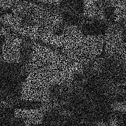
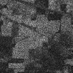
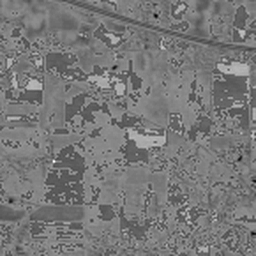
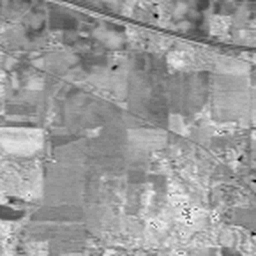
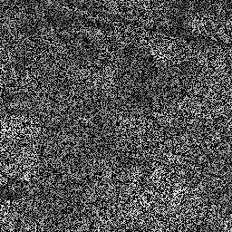
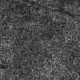
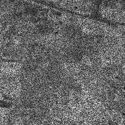
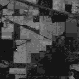
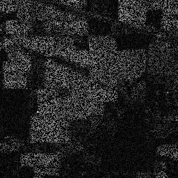
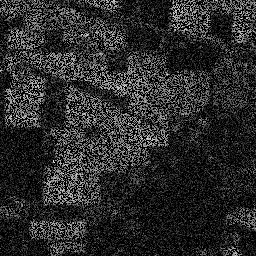
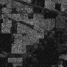
Reconstruction Gallery — 4 Scenes × 3 Scenarios
Method: CPU_baseline | Mismatch: nominal (nominal=True, perturbed=False)
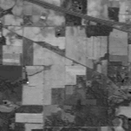
Ground Truth

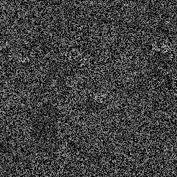
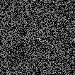
Measurement
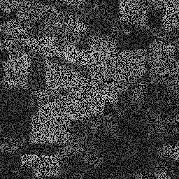
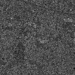
Reconstruction
Ground Truth

Measurement
Reconstruction
Ground Truth
Measurement (perturbed)
Reconstruction


Mean PSNR Across All Scenes
Per-scene PSNR breakdown (4 scenes)
| Scene | I (PSNR) | I (SSIM) | II (PSNR) | II (SSIM) | III (PSNR) | III (SSIM) |
|---|---|---|---|---|---|---|
| scene_00 | 10.250508893567286 | 0.06513993296399861 | 10.575776978929575 | 0.06865571587147419 | 13.5588212758422 | 0.15079016986433963 |
| scene_01 | 9.591961218151473 | 0.05945581635167391 | 9.847798943447778 | 0.06119383834938057 | 12.703534917938157 | 0.14941227753358832 |
| scene_02 | 7.267486903689603 | 0.031108077408166193 | 7.488631436864621 | 0.03629625685096665 | 10.740995171531333 | 0.0940621093423505 |
| scene_03 | 13.75776189776936 | 0.19370261836058633 | 13.709566684910302 | 0.1417126151074191 | 16.730848087228505 | 0.25759159954482574 |
| Mean | 10.216929728294431 | 0.08735161127110626 | 10.405443511038069 | 0.07696460654481013 | 13.433549863135049 | 0.16296403907127605 |
Experimental Setup
Key References
- Candes et al., 'Robust uncertainty principles: exact signal reconstruction from highly incomplete frequency information', IEEE TIT 52, 489-509 (2006)
- Donoho, 'Compressed sensing', IEEE TIT 52, 1289-1306 (2006)
Canonical Datasets
- Set11 / BSD68 (simulation benchmarks)
Spec DAG — Forward Model Pipeline
M(Φ) → D(g, η₁)
Mismatch Parameters
| Symbol | Parameter | Description | Nominal | Perturbed |
|---|---|---|---|---|
| ΔΦ | matrix_perturb | Matrix element perturbation std | 0 | 0.01 |
| g | gain | Detector gain multiplier | 1.0 | 1.03 |
| σ_y | sigma_y | Measurement noise std | 0 | 0.02 |
Credits System
Spec Primitives Reference (11 primitives)
Free-space or medium propagation kernel (Fresnel, Rayleigh-Sommerfeld).
Spatial or spatio-temporal amplitude modulation (coded aperture, SLM pattern).
Geometric projection operator (Radon transform, fan-beam, cone-beam).
Sampling in the Fourier / k-space domain (MRI, ptychography).
Shift-invariant convolution with a point-spread function (PSF).
Summation along a physical dimension (spectral, temporal, angular).
Sensor readout with gain g and noise model η (Gaussian, Poisson, mixed).
Patterned illumination (block, Hadamard, random) applied to the scene.
Spectral dispersion element (prism, grating) with shift α and aperture a.
Sample or gantry rotation (CT, electron tomography).
Spectral filter or monochromator selecting a wavelength band.