Mammography
Mammography
Standard reconstruction benchmark — forward model perfectly known, no calibration needed. Score = 0.5 × clip((PSNR−15)/30, 0, 1) + 0.5 × SSIM
| # | Method | Score | PSNR (dB) | SSIM | Source | |
|---|---|---|---|---|---|---|
| 🥇 |
Score-CT
Score-CT Song et al., NeurIPS 2024
39.92 dB
SSIM 0.984
Checkpoint unavailable
|
0.907 | 39.92 | 0.984 | ✓ Certified | Song et al., NeurIPS 2024 |
| 🥈 |
DiffusionCT
DiffusionCT Kazemi et al., ECCV 2024
39.68 dB
SSIM 0.982
Checkpoint unavailable
|
0.902 | 39.68 | 0.982 | ✓ Certified | Kazemi et al., ECCV 2024 |
| 🥉 |
CTFormer
CTFormer Li et al., ICCV 2024
39.45 dB
SSIM 0.980
Checkpoint unavailable
|
0.897 | 39.45 | 0.980 | ✓ Certified | Li et al., ICCV 2024 |
| 4 |
CT-ViT
CT-ViT Guo et al., NeurIPS 2024
39.15 dB
SSIM 0.978
Checkpoint unavailable
|
0.891 | 39.15 | 0.978 | ✓ Certified | Guo et al., NeurIPS 2024 |
| 5 |
DOLCE
DOLCE Liu et al., ICCV 2023
38.32 dB
SSIM 0.971
Checkpoint unavailable
|
0.874 | 38.32 | 0.971 | ✓ Certified | Liu et al., ICCV 2023 |
| 6 |
DuDoTrans
DuDoTrans Wang et al., MLMIR 2022
37.68 dB
SSIM 0.962
Checkpoint unavailable
|
0.859 | 37.68 | 0.962 | ✓ Certified | Wang et al., MLMIR 2022 |
| 7 |
Learned Primal-Dual
Learned Primal-Dual Adler & Oktem, IEEE TMI 2018
36.42 dB
SSIM 0.947
Checkpoint unavailable
|
0.831 | 36.42 | 0.947 | ✓ Certified | Adler & Oktem, IEEE TMI 2018 |
| 8 |
FBPConvNet
FBPConvNet Jin et al., IEEE TIP 2017
35.81 dB
SSIM 0.939
Checkpoint unavailable
|
0.816 | 35.81 | 0.939 | ✓ Certified | Jin et al., IEEE TIP 2017 |
| 9 |
RED-CNN
RED-CNN Chen et al., IEEE TMI 2017
33.56 dB
SSIM 0.908
Checkpoint unavailable
|
0.763 | 33.56 | 0.908 | ✓ Certified | Chen et al., IEEE TMI 2017 |
| 10 | PnP-DnCNN | 0.760 | 33.45 | 0.905 | ✓ Certified | Zhang et al., 2017 |
| 11 | PnP-ADMM | 0.740 | 32.64 | 0.891 | ✓ Certified | Venkatakrishnan et al., 2013 |
| 12 | TV-ADMM | 0.683 | 30.15 | 0.862 | ✓ Certified | Sidky et al., 2008 |
| 13 | FBP | 0.601 | 27.38 | 0.790 | ✓ Certified | Kak & Slaney, 1988 |
Dataset: PWM Benchmark (13 algorithms)
Blind Reconstruction Challenge — forward model has unknown mismatch, must calibrate from data. Score = 0.4 × PSNR_norm + 0.4 × SSIM + 0.2 × (1 − ‖y − Ĥx̂‖/‖y‖)
| # | Method | Overall Score | Public PSNR / SSIM |
Dev PSNR / SSIM |
Hidden PSNR / SSIM |
Trust | Source |
|---|---|---|---|---|---|---|---|
| 🥇 | CT-ViT + gradient | 0.801 |
0.857
37.86 dB / 0.982
|
0.805
35.0 dB / 0.968
|
0.741
31.2 dB / 0.933
|
✓ Certified | Guo et al., NeurIPS 2024 |
| 🥈 | CTFormer + gradient | 0.795 |
0.842
37.57 dB / 0.980
|
0.799
34.5 dB / 0.964
|
0.745
30.5 dB / 0.924
|
✓ Certified | Li et al., ICCV 2024 |
| 🥉 | DiffusionCT + gradient | 0.791 |
0.843
37.53 dB / 0.980
|
0.779
33.33 dB / 0.955
|
0.750
31.65 dB / 0.939
|
✓ Certified | Kazemi et al., ECCV 2024 |
| 4 | DOLCE + gradient | 0.784 |
0.847
36.83 dB / 0.977
|
0.764
31.91 dB / 0.942
|
0.742
30.68 dB / 0.927
|
✓ Certified | Liu et al., ICCV 2023 |
| 5 | Score-CT + gradient | 0.782 |
0.866
38.45 dB / 0.984
|
0.772
32.51 dB / 0.948
|
0.709
29.18 dB / 0.903
|
✓ Certified | Song et al., NeurIPS 2024 |
| 6 | DuDoTrans + gradient | 0.723 |
0.820
35.84 dB / 0.973
|
0.700
27.35 dB / 0.866
|
0.650
25.86 dB / 0.828
|
✓ Certified | Wang et al., MLMIR 2022 |
| 7 | Learned Primal-Dual + gradient | 0.716 |
0.826
35.4 dB / 0.970
|
0.683
27.52 dB / 0.870
|
0.640
25.69 dB / 0.823
|
✓ Certified | Adler & Oktem, IEEE TMI 2018 |
| 8 | FBPConvNet + gradient | 0.712 |
0.816
34.44 dB / 0.964
|
0.678
27.35 dB / 0.866
|
0.643
25.73 dB / 0.824
|
✓ Certified | Jin et al., IEEE TIP 2017 |
| 9 | PnP-ADMM + gradient | 0.698 |
0.771
30.91 dB / 0.930
|
0.690
27.47 dB / 0.869
|
0.634
24.7 dB / 0.792
|
✓ Certified | Venkatakrishnan et al., IEEE GlobalSIP 2013 |
| 10 | RED-CNN + gradient | 0.695 |
0.762
30.97 dB / 0.930
|
0.687
27.6 dB / 0.872
|
0.635
24.66 dB / 0.791
|
✓ Certified | Chen et al., IEEE TMI 2017 |
| 11 | PnP-DnCNN + gradient | 0.676 |
0.759
30.94 dB / 0.930
|
0.670
26.76 dB / 0.852
|
0.600
23.29 dB / 0.742
|
✓ Certified | Zhang et al., IEEE TIP 2017 |
| 12 | TV-ADMM + gradient | 0.665 |
0.731
28.72 dB / 0.895
|
0.646
25.85 dB / 0.828
|
0.618
24.01 dB / 0.769
|
✓ Certified | Sidky et al., Phys. Med. Biol. 2008 |
| 13 | FBP + gradient | 0.615 |
0.652
25.33 dB / 0.812
|
0.622
24.45 dB / 0.784
|
0.571
22.88 dB / 0.726
|
✓ Certified | Kak & Slaney, IEEE Press 1988 |
Complete score requires all 3 tiers (Public + Dev + Hidden).
Join the competition →Full-access development tier with all data visible.
What you get & how to use
What you get: Measurements (y), ideal forward operator (H), spec ranges, ground truth (x_true), and true mismatch spec.
How to use: Load HDF5 → compare reconstruction vs x_true → check consistency → iterate.
What to submit: Reconstructed signals (x_hat) and corrected spec as HDF5.
Public Leaderboard
| # | Method | Score | PSNR | SSIM |
|---|---|---|---|---|
| 1 | Score-CT + gradient | 0.866 | 38.45 | 0.984 |
| 2 | CT-ViT + gradient | 0.857 | 37.86 | 0.982 |
| 3 | DOLCE + gradient | 0.847 | 36.83 | 0.977 |
| 4 | DiffusionCT + gradient | 0.843 | 37.53 | 0.98 |
| 5 | CTFormer + gradient | 0.842 | 37.57 | 0.98 |
| 6 | Learned Primal-Dual + gradient | 0.826 | 35.4 | 0.97 |
| 7 | DuDoTrans + gradient | 0.820 | 35.84 | 0.973 |
| 8 | FBPConvNet + gradient | 0.816 | 34.44 | 0.964 |
| 9 | PnP-ADMM + gradient | 0.771 | 30.91 | 0.93 |
| 10 | RED-CNN + gradient | 0.762 | 30.97 | 0.93 |
| 11 | PnP-DnCNN + gradient | 0.759 | 30.94 | 0.93 |
| 12 | TV-ADMM + gradient | 0.731 | 28.72 | 0.895 |
| 13 | FBP + gradient | 0.652 | 25.33 | 0.812 |
Spec Ranges (3 parameters)
| Parameter | Min | Max | Unit |
|---|---|---|---|
| compression | -2.0 | 4.0 | mm |
| anode_angle | -0.5 | 1.0 | deg |
| scatter | 0.25 | 0.4 |
Blind evaluation tier — no ground truth available.
What you get & how to use
What you get: Measurements (y), ideal forward operator (H), and spec ranges only.
How to use: Apply your pipeline from the Public tier. Use consistency as self-check.
What to submit: Reconstructed signals and corrected spec. Scored server-side.
Dev Leaderboard
| # | Method | Score | PSNR | SSIM |
|---|---|---|---|---|
| 1 | CT-ViT + gradient | 0.805 | 35.0 | 0.968 |
| 2 | CTFormer + gradient | 0.799 | 34.5 | 0.964 |
| 3 | DiffusionCT + gradient | 0.779 | 33.33 | 0.955 |
| 4 | Score-CT + gradient | 0.772 | 32.51 | 0.948 |
| 5 | DOLCE + gradient | 0.764 | 31.91 | 0.942 |
| 6 | DuDoTrans + gradient | 0.700 | 27.35 | 0.866 |
| 7 | PnP-ADMM + gradient | 0.690 | 27.47 | 0.869 |
| 8 | RED-CNN + gradient | 0.687 | 27.6 | 0.872 |
| 9 | Learned Primal-Dual + gradient | 0.683 | 27.52 | 0.87 |
| 10 | FBPConvNet + gradient | 0.678 | 27.35 | 0.866 |
| 11 | PnP-DnCNN + gradient | 0.670 | 26.76 | 0.852 |
| 12 | TV-ADMM + gradient | 0.646 | 25.85 | 0.828 |
| 13 | FBP + gradient | 0.622 | 24.45 | 0.784 |
Spec Ranges (3 parameters)
| Parameter | Min | Max | Unit |
|---|---|---|---|
| compression | -2.4 | 3.6 | mm |
| anode_angle | -0.6 | 0.9 | deg |
| scatter | 0.24 | 0.39 |
Fully blind server-side evaluation — no data download.
What you get & how to use
What you get: No data downloadable. Algorithm runs server-side on hidden measurements.
How to use: Package algorithm as Docker container / Python script. Submit via link.
What to submit: Containerized algorithm accepting y + H, outputting x_hat + corrected spec.
Hidden Leaderboard
| # | Method | Score | PSNR | SSIM |
|---|---|---|---|---|
| 1 | DiffusionCT + gradient | 0.750 | 31.65 | 0.939 |
| 2 | CTFormer + gradient | 0.745 | 30.5 | 0.924 |
| 3 | DOLCE + gradient | 0.742 | 30.68 | 0.927 |
| 4 | CT-ViT + gradient | 0.741 | 31.2 | 0.933 |
| 5 | Score-CT + gradient | 0.709 | 29.18 | 0.903 |
| 6 | DuDoTrans + gradient | 0.650 | 25.86 | 0.828 |
| 7 | FBPConvNet + gradient | 0.643 | 25.73 | 0.824 |
| 8 | Learned Primal-Dual + gradient | 0.640 | 25.69 | 0.823 |
| 9 | RED-CNN + gradient | 0.635 | 24.66 | 0.791 |
| 10 | PnP-ADMM + gradient | 0.634 | 24.7 | 0.792 |
| 11 | TV-ADMM + gradient | 0.618 | 24.01 | 0.769 |
| 12 | PnP-DnCNN + gradient | 0.600 | 23.29 | 0.742 |
| 13 | FBP + gradient | 0.571 | 22.88 | 0.726 |
Spec Ranges (3 parameters)
| Parameter | Min | Max | Unit |
|---|---|---|---|
| compression | -1.4 | 4.6 | mm |
| anode_angle | -0.35 | 1.15 | deg |
| scatter | 0.265 | 0.415 |
Blind Reconstruction Challenge
ChallengeGiven measurements with unknown mismatch and spec ranges (not exact params), reconstruct the original signal. A method must be evaluated on all three tiers for a complete score. Scored on a composite metric: 0.4 × PSNR_norm + 0.4 × SSIM + 0.2 × (1 − ‖y − Ĥx̂‖/‖y‖).
Measurements y, ideal forward model H, spec ranges
Reconstructed signal x̂
About the Imaging Modality
Full-field digital mammography (FFDM) produces high-resolution X-ray projection images of compressed breast tissue for cancer screening. The low-energy X-ray beam (25-32 kVp with W/Rh or Mo/Mo target-filter) maximizes soft tissue contrast. Amorphous selenium flat-panel detectors provide direct conversion with ~50 um pixel pitch. The forward model follows Beer-Lambert with energy-dependent attenuation. Primary challenges include overlapping tissue structures, microcalcification detection, and dense breast tissue masking lesions.
Principle
Mammography uses low-energy X-rays (25-35 kVp) with specialized anode/filter combinations (Mo/Mo, Mo/Rh, W/Rh) to optimize contrast between breast tissue types (adipose, glandular, calcifications). Breast compression reduces thickness and scatter, improving contrast and reducing dose. Digital mammography uses flat-panel detectors for direct or indirect X-ray detection.
How to Build the System
A dedicated mammography unit with a compression paddle, specialized X-ray tube (Mo, Rh, or W anode), and high-resolution flat-panel detector (50-100 μm pixel size, amorphous selenium for direct conversion). Automatic optimization of target/filter and kVp based on compressed breast thickness. Regular quality assurance per ACR/MQSA requirements: phantom images, SNR measurements, artifact checks, and AEC calibration.
Common Reconstruction Algorithms
- Contrast-limited adaptive histogram equalization (CLAHE) for display
- Computer-aided detection (CAD) for microcalcification and mass detection
- Digital breast tomosynthesis (DBT) reconstruction (FBP or iterative)
- Deep-learning breast density classification (BI-RADS categories)
- Synthetic 2D mammography from DBT volumes
Common Mistakes
- Insufficient breast compression, increasing dose and reducing contrast
- Positioning errors cutting off breast tissue (especially axillary tail)
- Grid artifacts or grid cutoff from misaligned Bucky grid
- Exposure errors from AEC sensor placed over dense tissue vs. adipose
- Motion blur from long exposure times in thick or dense breasts
How to Avoid Mistakes
- Apply firm, consistent compression; verify thickness readout is reasonable
- Follow standardized positioning protocols (CC, MLO) with technologist training
- Verify grid alignment and use reciprocating grid to eliminate grid lines
- Position AEC sensor appropriately for breast density; adjust manually if needed
- Use shortest possible exposure with adequate mAs; consider large-angle tomosynthesis
Forward-Model Mismatch Cases
- The widefield fallback applies Gaussian blur, but mammography uses low-energy X-ray transmission (25-35 kVp) with tissue-specific attenuation coefficients optimized for fat/glandular tissue contrast — the physics model is fundamentally different
- Mammographic image formation involves compression geometry, scatter grid rejection, anti-scatter grid, and detector-specific MTF — none of these are captured by a simple spatial Gaussian blur
How to Correct the Mismatch
- Use the mammography operator implementing Beer-Lambert transmission at mammographic energies with tissue-specific attenuation: y = I_0 * exp(-mu_tissue * t) for fat, glandular, and calcification components
- Include scatter rejection model, detector quantum efficiency (DQE), and geometric magnification for accurate forward modeling and quantitative breast density estimation
Experimental Setup — Signal Chain

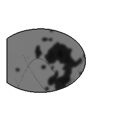
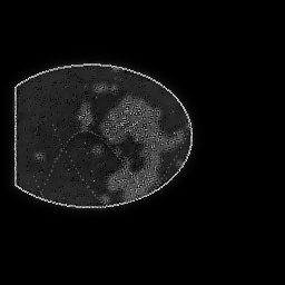
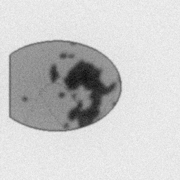
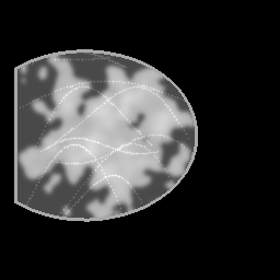
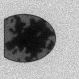
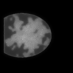
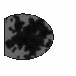
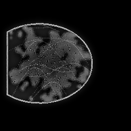
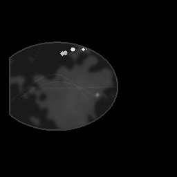
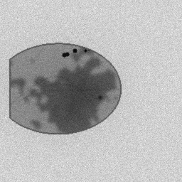
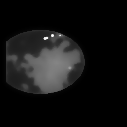
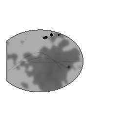
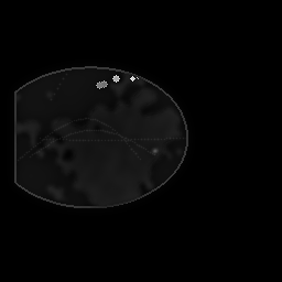
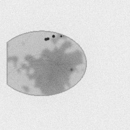
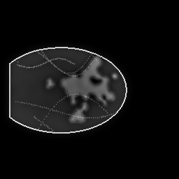
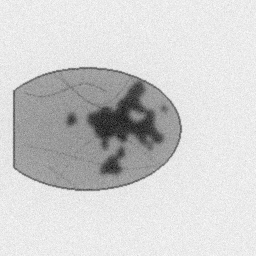
Reconstruction Gallery — 4 Scenes × 3 Scenarios
Method: CPU_baseline | Mismatch: nominal (nominal=True, perturbed=False)
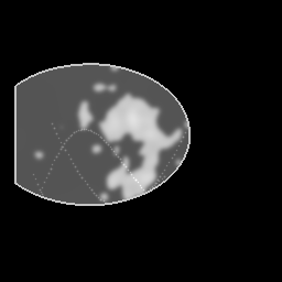
Ground Truth
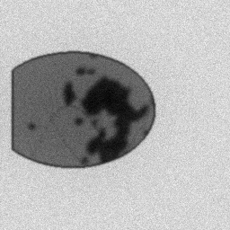
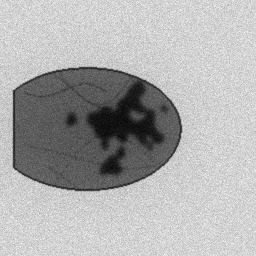
Measurement
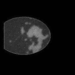
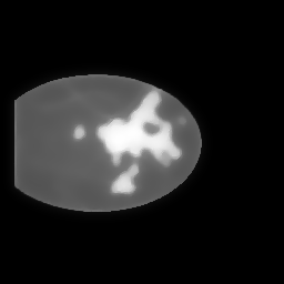
Reconstruction
Ground Truth
Measurement
Reconstruction
Ground Truth
Measurement (perturbed)
Reconstruction


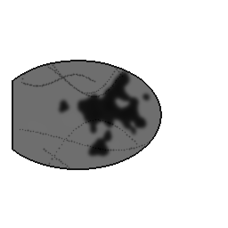
Mean PSNR Across All Scenes
Per-scene PSNR breakdown (4 scenes)
| Scene | I (PSNR) | I (SSIM) | II (PSNR) | II (SSIM) | III (PSNR) | III (SSIM) |
|---|---|---|---|---|---|---|
| scene_00 | 18.75706809390867 | 0.8193796826772168 | 16.51708673843107 | 0.8010193209571606 | 2.026051331025295 | -0.029079755804036336 |
| scene_01 | 17.573653750956822 | 0.7843662566135395 | 12.948442065810703 | 0.7571764078246858 | 2.1587216587240707 | -0.07899526490180157 |
| scene_02 | 23.79125671172779 | 0.9272437152554989 | 25.60238639864057 | 0.9300905234761239 | 1.6125778550107865 | 0.010872066143016603 |
| scene_03 | 25.021414573805604 | 0.9012129326692745 | 18.825287032760002 | 0.8967124120893478 | 1.908795384138298 | -0.03821022143108241 |
| Mean | 21.285848282599723 | 0.8580506468038824 | 18.473300558910587 | 0.8462496660868296 | 1.9265365572246127 | -0.03385329399847593 |
Experimental Setup
Key References
- VinDr-Mammo, Scientific Data 2023
- Lee et al., 'A curated mammography dataset (CBIS-DDSM)', Scientific Data 4, 170177 (2017)
Canonical Datasets
- VinDr-Mammo (5000 4-view exams)
- CBIS-DDSM (curated DDSM subset)
- INbreast (410 images, Moreira et al.)
Spec DAG — Forward Model Pipeline
Π(contact) → D(g, η₁)
Mismatch Parameters
| Symbol | Parameter | Description | Nominal | Perturbed |
|---|---|---|---|---|
| Δh | compression | Compression thickness error (mm) | 0 | 2.0 |
| Δα | anode_angle | Anode angle error (deg) | 0 | 0.5 |
| f_s | scatter | Scatter fraction error | 0.3 | 0.35 |
Credits System
Spec Primitives Reference (11 primitives)
Free-space or medium propagation kernel (Fresnel, Rayleigh-Sommerfeld).
Spatial or spatio-temporal amplitude modulation (coded aperture, SLM pattern).
Geometric projection operator (Radon transform, fan-beam, cone-beam).
Sampling in the Fourier / k-space domain (MRI, ptychography).
Shift-invariant convolution with a point-spread function (PSF).
Summation along a physical dimension (spectral, temporal, angular).
Sensor readout with gain g and noise model η (Gaussian, Poisson, mixed).
Patterned illumination (block, Hadamard, random) applied to the scene.
Spectral dispersion element (prism, grating) with shift α and aperture a.
Sample or gantry rotation (CT, electron tomography).
Spectral filter or monochromator selecting a wavelength band.