Light-Sheet
Light-Sheet Fluorescence Microscopy
Standard reconstruction benchmark — forward model perfectly known, no calibration needed. Score = 0.5 × clip((PSNR−15)/30, 0, 1) + 0.5 × SSIM
| # | Method | Score | PSNR (dB) | SSIM | Source | |
|---|---|---|---|---|---|---|
| 🥇 |
ScoreMicro
ScoreMicro Wei et al., ECCV 2025
38.48 dB
SSIM 0.981
Checkpoint unavailable
|
0.882 | 38.48 | 0.981 | ✓ Certified | Wei et al., ECCV 2025 |
| 🥈 |
DiffDeconv
DiffDeconv Huang et al., NeurIPS 2024
38.12 dB
SSIM 0.979
Checkpoint unavailable
|
0.875 | 38.12 | 0.979 | ✓ Certified | Huang et al., NeurIPS 2024 |
| 🥉 |
Restormer+
Restormer+ Zamir et al., ICCV 2024
37.65 dB
SSIM 0.975
Checkpoint unavailable
|
0.865 | 37.65 | 0.975 | ✓ Certified | Zamir et al., ICCV 2024 |
| 4 |
DeconvFormer
DeconvFormer Chen et al., CVPR 2024
37.25 dB
SSIM 0.972
Checkpoint unavailable
|
0.857 | 37.25 | 0.972 | ✓ Certified | Chen et al., CVPR 2024 |
| 5 |
ResUNet
ResUNet DeCelle et al., Nat. Methods 2021
35.85 dB
SSIM 0.964
Checkpoint unavailable
|
0.830 | 35.85 | 0.964 | ✓ Certified | DeCelle et al., Nat. Methods 2021 |
| 6 |
Restormer
Restormer Zamir et al., CVPR 2022
35.8 dB
SSIM 0.962
Checkpoint unavailable
|
0.828 | 35.8 | 0.962 | ✓ Certified | Zamir et al., CVPR 2022 |
| 7 |
U-Net
U-Net Ronneberger et al., MICCAI 2015
35.15 dB
SSIM 0.956
Checkpoint unavailable
|
0.814 | 35.15 | 0.956 | ✓ Certified | Ronneberger et al., MICCAI 2015 |
| 8 |
CARE
CARE Weigert et al., Nat. Methods 2018
34.5 dB
SSIM 0.948
Checkpoint unavailable
|
0.799 | 34.5 | 0.948 | ✓ Certified | Weigert et al., Nat. Methods 2018 |
| 9 | PnP-DnCNN | 0.715 | 31.2 | 0.890 | ✓ Certified | Zhang et al., IEEE TIP 2017 |
| 10 | PnP-FISTA | 0.693 | 30.42 | 0.872 | ✓ Certified | Bai et al., 2020 |
| 11 | TV-Deconvolution | 0.664 | 29.5 | 0.845 | ✓ Certified | TV-regularized deconvolution |
| 12 | Wiener Filter | 0.625 | 28.35 | 0.805 | ✓ Certified | Analytical baseline |
| 13 | Richardson-Lucy | 0.587 | 27.1 | 0.770 | ✓ Certified | Richardson 1972 / Lucy 1974 |
Dataset: PWM Benchmark (13 algorithms)
Blind Reconstruction Challenge — forward model has unknown mismatch, must calibrate from data. Score = 0.4 × PSNR_norm + 0.4 × SSIM + 0.2 × (1 − ‖y − Ĥx̂‖/‖y‖)
| # | Method | Overall Score | Public PSNR / SSIM |
Dev PSNR / SSIM |
Hidden PSNR / SSIM |
Trust | Source |
|---|---|---|---|---|---|---|---|
| 🥇 | Restormer+ + gradient | 0.785 |
0.838
36.04 dB / 0.974
|
0.771
33.17 dB / 0.954
|
0.746
31.11 dB / 0.932
|
✓ Certified | Zamir et al., ICCV 2024 |
| 🥈 | ScoreMicro + gradient | 0.780 |
0.848
36.73 dB / 0.977
|
0.758
31.1 dB / 0.932
|
0.733
30.4 dB / 0.923
|
✓ Certified | Wei et al., ECCV 2025 |
| 🥉 | Restormer + gradient | 0.773 |
0.818
34.77 dB / 0.966
|
0.769
31.55 dB / 0.938
|
0.733
30.38 dB / 0.922
|
✓ Certified | Zamir et al., CVPR 2022 |
| 4 | DeconvFormer + gradient | 0.772 |
0.834
36.06 dB / 0.974
|
0.772
32.8 dB / 0.951
|
0.710
29.7 dB / 0.912
|
✓ Certified | Chen et al., CVPR 2024 |
| 5 | DiffDeconv + gradient | 0.754 |
0.822
35.58 dB / 0.971
|
0.734
30.32 dB / 0.922
|
0.705
28.59 dB / 0.893
|
✓ Certified | Huang et al., NeurIPS 2024 |
| 6 | ResUNet + gradient | 0.726 |
0.794
33.36 dB / 0.956
|
0.722
29.19 dB / 0.904
|
0.662
26.14 dB / 0.836
|
✓ Certified | DeCelle et al., Nat. Methods 2021 |
| 7 | U-Net + gradient | 0.720 |
0.806
33.52 dB / 0.957
|
0.697
28.25 dB / 0.886
|
0.656
26.43 dB / 0.844
|
✓ Certified | Ronneberger et al., MICCAI 2015 |
| 8 | CARE + gradient | 0.710 |
0.778
32.35 dB / 0.946
|
0.700
27.55 dB / 0.871
|
0.653
26.28 dB / 0.840
|
✓ Certified | Weigert et al., Nat. Methods 2018 |
| 9 | PnP-DnCNN + gradient | 0.700 |
0.748
29.56 dB / 0.910
|
0.682
26.65 dB / 0.849
|
0.670
26.62 dB / 0.849
|
✓ Certified | Zhang et al., IEEE TIP 2017 |
| 10 | TV-Deconvolution + gradient | 0.677 |
0.719
27.81 dB / 0.877
|
0.663
26.67 dB / 0.850
|
0.649
26.12 dB / 0.835
|
✓ Certified | Rudin et al., Phys. A 1992 |
| 11 | PnP-FISTA + gradient | 0.643 |
0.736
28.75 dB / 0.896
|
0.629
24.21 dB / 0.776
|
0.564
22.44 dB / 0.708
|
✓ Certified | Bai et al., 2020 |
| 12 | Wiener Filter + gradient | 0.625 |
0.662
25.43 dB / 0.815
|
0.606
23.44 dB / 0.748
|
0.606
23.87 dB / 0.764
|
✓ Certified | Analytical baseline |
| 13 |
Richardson-Lucy + gradient
Richardson-Lucy + gradient Richardson, JOSA 1972 / Lucy, AJ 1974 Score 0.607
Correct & Reconstruct →
|
0.607 |
0.650
25.3 dB / 0.812
|
0.599
23.17 dB / 0.738
|
0.572
22.13 dB / 0.696
|
✓ Certified | Richardson, JOSA 1972 / Lucy, AJ 1974 |
Complete score requires all 3 tiers (Public + Dev + Hidden).
Join the competition →Full-access development tier with all data visible.
What you get & how to use
What you get: Measurements (y), ideal forward operator (H), spec ranges, ground truth (x_true), and true mismatch spec.
How to use: Load HDF5 → compare reconstruction vs x_true → check consistency → iterate.
What to submit: Reconstructed signals (x_hat) and corrected spec as HDF5.
Public Leaderboard
| # | Method | Score | PSNR | SSIM |
|---|---|---|---|---|
| 1 | ScoreMicro + gradient | 0.848 | 36.73 | 0.977 |
| 2 | Restormer+ + gradient | 0.838 | 36.04 | 0.974 |
| 3 | DeconvFormer + gradient | 0.834 | 36.06 | 0.974 |
| 4 | DiffDeconv + gradient | 0.822 | 35.58 | 0.971 |
| 5 | Restormer + gradient | 0.818 | 34.77 | 0.966 |
| 6 | U-Net + gradient | 0.806 | 33.52 | 0.957 |
| 7 | ResUNet + gradient | 0.794 | 33.36 | 0.956 |
| 8 | CARE + gradient | 0.778 | 32.35 | 0.946 |
| 9 | PnP-DnCNN + gradient | 0.748 | 29.56 | 0.91 |
| 10 | PnP-FISTA + gradient | 0.736 | 28.75 | 0.896 |
| 11 | TV-Deconvolution + gradient | 0.719 | 27.81 | 0.877 |
| 12 | Wiener Filter + gradient | 0.662 | 25.43 | 0.815 |
| 13 | Richardson-Lucy + gradient | 0.650 | 25.3 | 0.812 |
Spec Ranges (3 parameters)
| Parameter | Min | Max | Unit |
|---|---|---|---|
| sheet_thickness | -1.0 | 2.0 | μm |
| sheet_tilt | -0.5 | 1.0 | deg |
| stripe_artifact | -0.1 | 0.2 |
Blind evaluation tier — no ground truth available.
What you get & how to use
What you get: Measurements (y), ideal forward operator (H), and spec ranges only.
How to use: Apply your pipeline from the Public tier. Use consistency as self-check.
What to submit: Reconstructed signals and corrected spec. Scored server-side.
Dev Leaderboard
| # | Method | Score | PSNR | SSIM |
|---|---|---|---|---|
| 1 | DeconvFormer + gradient | 0.772 | 32.8 | 0.951 |
| 2 | Restormer+ + gradient | 0.771 | 33.17 | 0.954 |
| 3 | Restormer + gradient | 0.769 | 31.55 | 0.938 |
| 4 | ScoreMicro + gradient | 0.758 | 31.1 | 0.932 |
| 5 | DiffDeconv + gradient | 0.734 | 30.32 | 0.922 |
| 6 | ResUNet + gradient | 0.722 | 29.19 | 0.904 |
| 7 | CARE + gradient | 0.700 | 27.55 | 0.871 |
| 8 | U-Net + gradient | 0.697 | 28.25 | 0.886 |
| 9 | PnP-DnCNN + gradient | 0.682 | 26.65 | 0.849 |
| 10 | TV-Deconvolution + gradient | 0.663 | 26.67 | 0.85 |
| 11 | PnP-FISTA + gradient | 0.629 | 24.21 | 0.776 |
| 12 | Wiener Filter + gradient | 0.606 | 23.44 | 0.748 |
| 13 | Richardson-Lucy + gradient | 0.599 | 23.17 | 0.738 |
Spec Ranges (3 parameters)
| Parameter | Min | Max | Unit |
|---|---|---|---|
| sheet_thickness | -1.2 | 1.8 | μm |
| sheet_tilt | -0.6 | 0.9 | deg |
| stripe_artifact | -0.12 | 0.18 |
Fully blind server-side evaluation — no data download.
What you get & how to use
What you get: No data downloadable. Algorithm runs server-side on hidden measurements.
How to use: Package algorithm as Docker container / Python script. Submit via link.
What to submit: Containerized algorithm accepting y + H, outputting x_hat + corrected spec.
Hidden Leaderboard
| # | Method | Score | PSNR | SSIM |
|---|---|---|---|---|
| 1 | Restormer+ + gradient | 0.746 | 31.11 | 0.932 |
| 2 | ScoreMicro + gradient | 0.733 | 30.4 | 0.923 |
| 3 | Restormer + gradient | 0.733 | 30.38 | 0.922 |
| 4 | DeconvFormer + gradient | 0.710 | 29.7 | 0.912 |
| 5 | DiffDeconv + gradient | 0.705 | 28.59 | 0.893 |
| 6 | PnP-DnCNN + gradient | 0.670 | 26.62 | 0.849 |
| 7 | ResUNet + gradient | 0.662 | 26.14 | 0.836 |
| 8 | U-Net + gradient | 0.656 | 26.43 | 0.844 |
| 9 | CARE + gradient | 0.653 | 26.28 | 0.84 |
| 10 | TV-Deconvolution + gradient | 0.649 | 26.12 | 0.835 |
| 11 | Wiener Filter + gradient | 0.606 | 23.87 | 0.764 |
| 12 | Richardson-Lucy + gradient | 0.572 | 22.13 | 0.696 |
| 13 | PnP-FISTA + gradient | 0.564 | 22.44 | 0.708 |
Spec Ranges (3 parameters)
| Parameter | Min | Max | Unit |
|---|---|---|---|
| sheet_thickness | -0.7 | 2.3 | μm |
| sheet_tilt | -0.35 | 1.15 | deg |
| stripe_artifact | -0.07 | 0.23 |
Blind Reconstruction Challenge
ChallengeGiven measurements with unknown mismatch and spec ranges (not exact params), reconstruct the original signal. A method must be evaluated on all three tiers for a complete score. Scored on a composite metric: 0.4 × PSNR_norm + 0.4 × SSIM + 0.2 × (1 − ‖y − Ĥx̂‖/‖y‖).
Measurements y, ideal forward model H, spec ranges
Reconstructed signal x̂
About the Imaging Modality
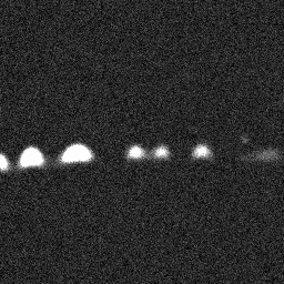
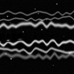
Light-sheet microscopy (LSFM / SPIM) illuminates the sample with a thin sheet of light perpendicular to the detection axis, providing intrinsic optical sectioning. Primary artifacts are stripe patterns caused by absorption and scattering in the illumination path, plus anisotropic PSF blur. The forward model is y = S(z) * (PSF_3d *** x) + n where S(z) models the stripe attenuation. Reconstruction involves destriping followed by optional deconvolution.
Principle
A thin sheet of laser light illuminates only the focal plane of the detection objective, providing intrinsic optical sectioning with minimal out-of-plane photobleaching. The orthogonal geometry between illumination and detection decouples sectioning from resolution. Detection is widefield, enabling fast volumetric imaging of large specimens.
How to Build the System
Arrange two orthogonal objective arms: one for the excitation sheet (cylindrical lens or digitally scanned Gaussian/Bessel beam) and one for detection (high-NA water-dipping). Mount the sample in agarose or hold in a chamber compatible with the dual-objective geometry. Use a fast sCMOS camera for detection. Stage scanning or sheet scanning acquires z-stacks. Consider diSPIM (dual-view) for isotropic resolution.
Common Reconstruction Algorithms
- Multi-view fusion (weighted averaging of complementary views)
- Multi-view deconvolution (Bayesian, joint Richardson-Lucy)
- Content-based image fusion
- Deep-learning denoising for high-speed acquisitions (CARE)
- Stripe artifact removal (wavelet-FFT filtering)
Common Mistakes
- Light sheet too thick, degrading axial resolution and sectioning
- Absorption and scattering in thick tissue causing shadow artifacts (stripes)
- Misalignment between sheet focal plane and detection focal plane
- Improper sample mounting causing drift or deformation during long acquisitions
- Ignoring refractive-index variations causing sheet deflection inside tissue
How to Avoid Mistakes
- Use Bessel or lattice light sheet for thin, uniform illumination profiles
- Pivot the light sheet or use dual-side illumination to reduce shadow artifacts
- Carefully co-align illumination and detection planes using fluorescent beads
- Use stable, low-melting-point agarose embedding and vibration-isolated stages
- Clear or match refractive index of tissue where possible; use adaptive optics
Forward-Model Mismatch Cases
- The widefield fallback processes only 2D (64,64) images, but light-sheet microscopy acquires 3D volumes (64,64,32) with intrinsic optical sectioning — the volumetric z-dimension is entirely lost
- Widefield illumination excites the entire sample volume causing out-of-focus blur, whereas the light sheet illuminates only the focal plane — the fallback forward model includes fluorescence contributions from planes that the real system never excites
How to Correct the Mismatch
- Use the lightsheet operator that processes 3D volumes with the sheet illumination profile: each z-slice is excited only by the thin (1-5 um) light sheet
- Model the sheet thickness and propagation (Gaussian or Bessel beam) explicitly; for multi-view systems, include the detection PSF from the orthogonal objective
Experimental Setup — Signal Chain

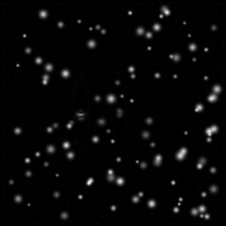
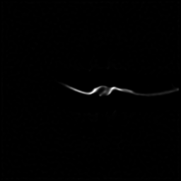
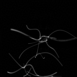
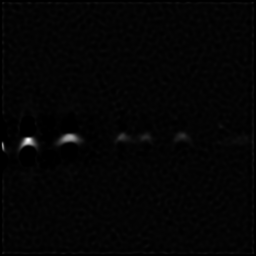
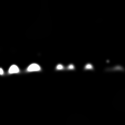
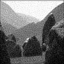
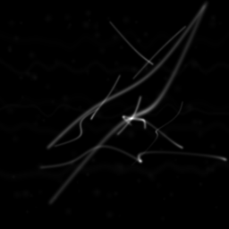
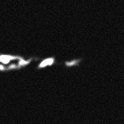
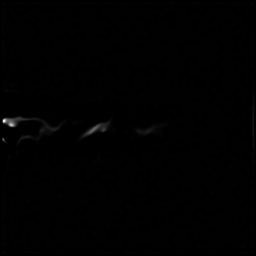
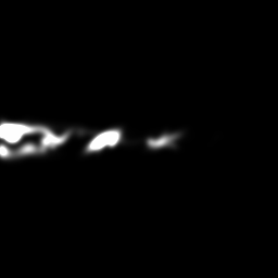
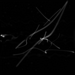
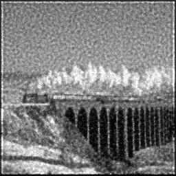
Reconstruction Gallery — 4 Scenes × 3 Scenarios
Method: CPU_baseline | Mismatch: nominal (nominal=True, perturbed=False)
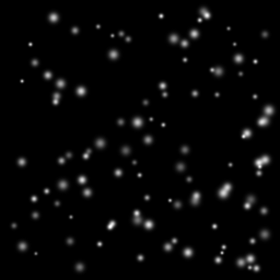
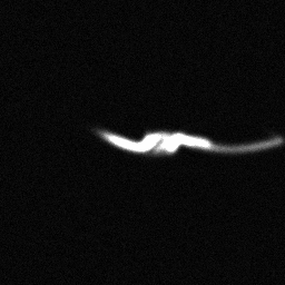
Ground Truth
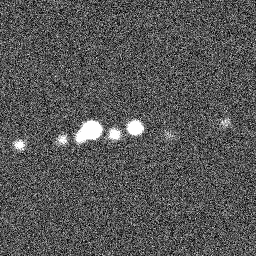
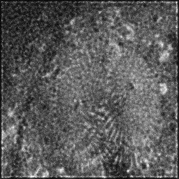
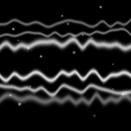
Measurement
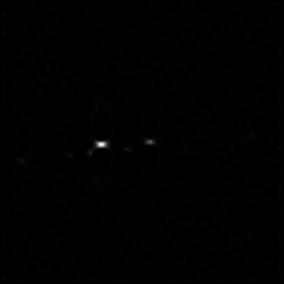
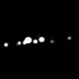
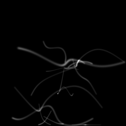
Reconstruction
Ground Truth
Measurement
Reconstruction
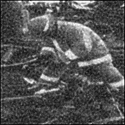
Ground Truth
Measurement (perturbed)
Reconstruction

Mean PSNR Across All Scenes
Per-scene PSNR breakdown (4 scenes)
| Scene | I (PSNR) | I (SSIM) | II (PSNR) | II (SSIM) | III (PSNR) | III (SSIM) |
|---|---|---|---|---|---|---|
| scene_00 | 20.0335822991388 | 0.6745269525732303 | 41.11067375476016 | 0.9298113249340058 | 8.593089342049813 | 0.0045005242056979965 |
| scene_01 | 27.624913705135235 | 0.8194840125975688 | 32.020699398087835 | 0.9126672495968701 | 8.640607029999796 | 0.001379776991637026 |
| scene_02 | 12.962241447100933 | 0.22194153105919903 | 31.085196541895836 | 0.6569434192039519 | 5.870863858966602 | 0.010240046462108887 |
| scene_03 | 26.20484422215066 | 0.7304966931968156 | 34.12566697991603 | 0.9348067589908261 | 5.679529011627023 | 0.006942560521091296 |
| Mean | 21.706395418381405 | 0.6116122973567034 | 34.58555916866497 | 0.8585571881814135 | 7.196022310660808 | 0.005765727045133801 |
Experimental Setup
Key References
- Huisken et al., 'Optical sectioning deep inside live embryos by SPIM', Science 305, 1007-1009 (2004)
- Power & Bhatt, 'A guide to light-sheet fluorescence microscopy for multiscale imaging', Nature Methods 14, 360-373 (2017)
Canonical Datasets
- OpenSPIM sample datasets
- Zebrafish developmental lightsheet atlas
Spec DAG — Forward Model Pipeline
C(PSF_sheet) → D(g, η₃)
Mismatch Parameters
| Symbol | Parameter | Description | Nominal | Perturbed |
|---|---|---|---|---|
| Δw | sheet_thickness | Sheet thickness error (μm) | 0 | 1.0 |
| Δθ | sheet_tilt | Sheet tilt (deg) | 0 | 0.5 |
| α_s | stripe_artifact | Stripe artifact amplitude | 0 | 0.1 |
Credits System
Spec Primitives Reference (11 primitives)
Free-space or medium propagation kernel (Fresnel, Rayleigh-Sommerfeld).
Spatial or spatio-temporal amplitude modulation (coded aperture, SLM pattern).
Geometric projection operator (Radon transform, fan-beam, cone-beam).
Sampling in the Fourier / k-space domain (MRI, ptychography).
Shift-invariant convolution with a point-spread function (PSF).
Summation along a physical dimension (spectral, temporal, angular).
Sensor readout with gain g and noise model η (Gaussian, Poisson, mixed).
Patterned illumination (block, Hadamard, random) applied to the scene.
Spectral dispersion element (prism, grating) with shift α and aperture a.
Sample or gantry rotation (CT, electron tomography).
Spectral filter or monochromator selecting a wavelength band.