Light Field
Light Field Imaging
Standard reconstruction benchmark — forward model perfectly known, no calibration needed. Score = 0.5 × clip((PSNR−15)/30, 0, 1) + 0.5 × SSIM
| # | Method | Score | PSNR (dB) | SSIM | Source | |
|---|---|---|---|---|---|---|
| 🥇 |
DistgSSR
DistgSSR Wang et al., CVPR 2022
35.5 dB
SSIM 0.948
Checkpoint unavailable
|
0.816 | 35.5 | 0.948 | ✓ Certified | Wang et al., CVPR 2022 |
| 🥈 |
LFNet
LFNet Wang et al., IEEE TPAMI 2020
33.0 dB
SSIM 0.915
Checkpoint unavailable
|
0.758 | 33.0 | 0.915 | ✓ Certified | Wang et al., IEEE TPAMI 2020 |
| 🥉 | PnP-LF | 0.635 | 28.5 | 0.820 | ✓ Certified | PnP-ADMM with angular prior |
| 4 | Shift-and-Sum | 0.503 | 24.5 | 0.690 | ✓ Certified | Ng et al., Stanford Tech Report 2005 |
Dataset: PWM Benchmark (4 algorithms)
Blind Reconstruction Challenge — forward model has unknown mismatch, must calibrate from data. Score = 0.4 × PSNR_norm + 0.4 × SSIM + 0.2 × (1 − ‖y − Ĥx̂‖/‖y‖)
| # | Method | Overall Score | Public PSNR / SSIM |
Dev PSNR / SSIM |
Hidden PSNR / SSIM |
Trust | Source |
|---|---|---|---|---|---|---|---|
| 🥇 | DistgSSR + gradient | 0.724 |
0.788
32.75 dB / 0.950
|
0.735
29.28 dB / 0.905
|
0.649
26.39 dB / 0.843
|
✓ Certified | Wang et al., CVPR 2022 |
| 🥈 | LFNet + gradient | 0.670 |
0.754
30.71 dB / 0.927
|
0.652
25.06 dB / 0.804
|
0.603
24.06 dB / 0.771
|
✓ Certified | Wang et al., IEEE TPAMI 2020 |
| 🥉 | PnP-LF + gradient | 0.552 |
0.666
25.58 dB / 0.820
|
0.521
20.34 dB / 0.615
|
0.470
18.61 dB / 0.530
|
✓ Certified | PnP-ADMM with angular prior |
| 4 | Shift-and-Sum + gradient | 0.534 |
0.578
22.16 dB / 0.697
|
0.534
20.52 dB / 0.623
|
0.489
19.65 dB / 0.582
|
✓ Certified | Ng et al., Stanford Tech Report 2005 |
Complete score requires all 3 tiers (Public + Dev + Hidden).
Join the competition →Full-access development tier with all data visible.
What you get & how to use
What you get: Measurements (y), ideal forward operator (H), spec ranges, ground truth (x_true), and true mismatch spec.
How to use: Load HDF5 → compare reconstruction vs x_true → check consistency → iterate.
What to submit: Reconstructed signals (x_hat) and corrected spec as HDF5.
Public Leaderboard
| # | Method | Score | PSNR | SSIM |
|---|---|---|---|---|
| 1 | DistgSSR + gradient | 0.788 | 32.75 | 0.95 |
| 2 | LFNet + gradient | 0.754 | 30.71 | 0.927 |
| 3 | PnP-LF + gradient | 0.666 | 25.58 | 0.82 |
| 4 | Shift-and-Sum + gradient | 0.578 | 22.16 | 0.697 |
Spec Ranges (3 parameters)
| Parameter | Min | Max | Unit |
|---|---|---|---|
| microlens_pitch | -0.5 | 1.0 | μm |
| main_lens_f | -0.1 | 0.2 | mm |
| vignetting | -3.0 | 6.0 | % |
Blind evaluation tier — no ground truth available.
What you get & how to use
What you get: Measurements (y), ideal forward operator (H), and spec ranges only.
How to use: Apply your pipeline from the Public tier. Use consistency as self-check.
What to submit: Reconstructed signals and corrected spec. Scored server-side.
Dev Leaderboard
| # | Method | Score | PSNR | SSIM |
|---|---|---|---|---|
| 1 | DistgSSR + gradient | 0.735 | 29.28 | 0.905 |
| 2 | LFNet + gradient | 0.652 | 25.06 | 0.804 |
| 3 | Shift-and-Sum + gradient | 0.534 | 20.52 | 0.623 |
| 4 | PnP-LF + gradient | 0.521 | 20.34 | 0.615 |
Spec Ranges (3 parameters)
| Parameter | Min | Max | Unit |
|---|---|---|---|
| microlens_pitch | -0.6 | 0.9 | μm |
| main_lens_f | -0.12 | 0.18 | mm |
| vignetting | -3.6 | 5.4 | % |
Fully blind server-side evaluation — no data download.
What you get & how to use
What you get: No data downloadable. Algorithm runs server-side on hidden measurements.
How to use: Package algorithm as Docker container / Python script. Submit via link.
What to submit: Containerized algorithm accepting y + H, outputting x_hat + corrected spec.
Hidden Leaderboard
| # | Method | Score | PSNR | SSIM |
|---|---|---|---|---|
| 1 | DistgSSR + gradient | 0.649 | 26.39 | 0.843 |
| 2 | LFNet + gradient | 0.603 | 24.06 | 0.771 |
| 3 | Shift-and-Sum + gradient | 0.489 | 19.65 | 0.582 |
| 4 | PnP-LF + gradient | 0.470 | 18.61 | 0.53 |
Spec Ranges (3 parameters)
| Parameter | Min | Max | Unit |
|---|---|---|---|
| microlens_pitch | -0.35 | 1.15 | μm |
| main_lens_f | -0.07 | 0.23 | mm |
| vignetting | -2.1 | 6.9 | % |
Blind Reconstruction Challenge
ChallengeGiven measurements with unknown mismatch and spec ranges (not exact params), reconstruct the original signal. A method must be evaluated on all three tiers for a complete score. Scored on a composite metric: 0.4 × PSNR_norm + 0.4 × SSIM + 0.2 × (1 − ‖y − Ĥx̂‖/‖y‖).
Measurements y, ideal forward model H, spec ranges
Reconstructed signal x̂
About the Imaging Modality
Light field imaging captures the full 4D radiance function L(x,y,u,v) describing both spatial position (x,y) and angular direction (u,v) of light rays. A microlens array placed before the sensor captures multiple sub-aperture views simultaneously, enabling post-capture refocusing, depth estimation, and perspective shifts. Each microlens images the objective's exit pupil, trading spatial resolution for angular resolution. The 4D light field can be processed with shift-and-sum for refocusing, disparity estimation for depth, or epipolar-plane image (EPI) analysis. Primary challenges include the inherent spatial-angular resolution tradeoff and microlens aberrations.
Principle
Light-field imaging captures both the spatial position and direction of light rays in a scene, recording a 4-D light field L(u,v,s,t) where (u,v) parameterize the aperture and (s,t) parameterize the spatial position. This enables computational refocusing, depth estimation, and novel viewpoint synthesis from a single capture. A microlens array placed before the sensor trades spatial resolution for angular resolution.
How to Build the System
Place a microlens array (MLA) at the sensor plane of a camera, one focal length in front of the image sensor. Each microlens captures the angular distribution of light from a corresponding spatial position (Lytro-style plenoptic camera). Alternative: use a camera array (e.g., 4×4 or 8×8 synchronized cameras) for higher angular and spatial resolution. Calibrate MLA alignment, microlens pitch, and main lens parameters.
Common Reconstruction Algorithms
- Shift-and-sum refocusing (synthetic aperture)
- Depth estimation from disparity between sub-aperture images
- Fourier slice theorem for light-field refocusing
- Light-field super-resolution (recovering spatial resolution lost to MLA)
- Deep-learning view synthesis (light field reconstruction from sparse views)
Common Mistakes
- Microlens array misaligned with sensor pixels, causing vignetting and crosstalk
- Insufficient angular samples for accurate depth estimation in textureless regions
- Not calibrating MLA-to-sensor alignment, producing decoding artifacts
- Confusing spatial and angular resolution trade-off limits of the plenoptic design
- Ignoring diffraction effects at the microlens apertures
How to Avoid Mistakes
- Precisely align MLA to sensor with sub-pixel accuracy; use calibration targets
- Increase camera array density or use coded-aperture techniques for more angular samples
- Calibrate using a white image and point-source images for precise microlens grid mapping
- Design the system with the desired spatial-angular trade-off explicitly computed
- Use microlens diameters larger than the diffraction limit (> 10× wavelength)
Forward-Model Mismatch Cases
- The widefield fallback produces a single (64,64) image, but a light field camera captures both spatial and angular information via a microlens array — the output encodes multiple sub-aperture views for computational refocusing
- Without the angular dimension (directions of light rays), depth estimation from parallax and computational refocusing are impossible — the widefield model captures only a single perspective
How to Correct the Mismatch
- Use the light field operator that models the microlens array: each microlens captures light from different angular directions, producing an (x, y, u, v) 4D light field on the 2D sensor
- Reconstruct depth maps from sub-aperture disparity, perform computational refocusing via shift-and-sum, or apply light-field super-resolution to trade angular for spatial resolution
Experimental Setup — Signal Chain

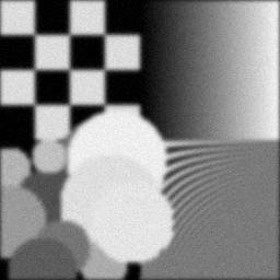
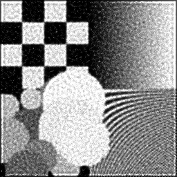
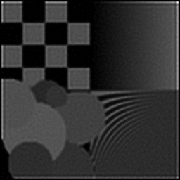
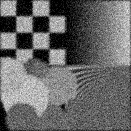
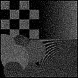
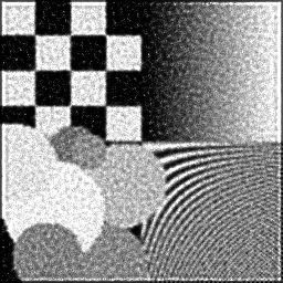
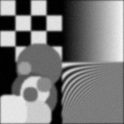
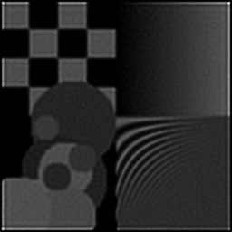
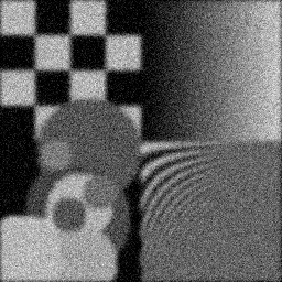
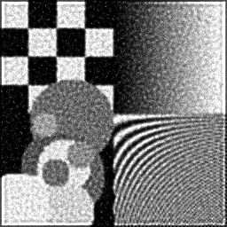
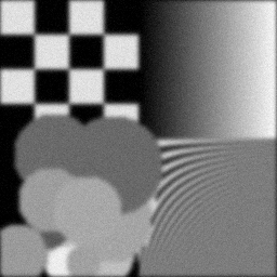
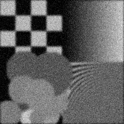
Reconstruction Gallery — 4 Scenes × 3 Scenarios
Method: CPU_baseline | Mismatch: nominal (nominal=True, perturbed=False)

Ground Truth
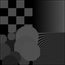
Measurement
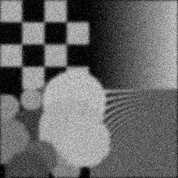
Reconstruction
Ground Truth
Measurement
Reconstruction
Ground Truth
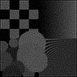
Measurement (perturbed)
Reconstruction


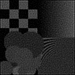

Mean PSNR Across All Scenes
Per-scene PSNR breakdown (4 scenes)
| Scene | I (PSNR) | I (SSIM) | II (PSNR) | II (SSIM) | III (PSNR) | III (SSIM) |
|---|---|---|---|---|---|---|
| scene_00 | 6.831755145049858 | 0.39251757962307293 | 6.747744781788927 | 0.19624154301519284 | 17.0733092814934 | 0.34599733923876136 |
| scene_01 | 7.208081904434112 | 0.39392374023822935 | 7.395701051446139 | 0.19865145380844743 | 16.91778445629049 | 0.35342995245672976 |
| scene_02 | 7.675436503843393 | 0.39375468365060645 | 7.1143972480104045 | 0.20103810356474872 | 16.88449427499023 | 0.37603178319129643 |
| scene_03 | 7.8398378914912294 | 0.39507824343020287 | 7.670146776544666 | 0.1976384681380463 | 16.96130682502457 | 0.341813373374832 |
| Mean | 7.388777861204648 | 0.39381856173552793 | 7.231997464447534 | 0.1983923921316088 | 16.959223709449674 | 0.35431811206540487 |
Experimental Setup
Key References
- Levoy & Hanrahan, 'Light field rendering', SIGGRAPH 1996
- Ng et al., 'Light field photography with a hand-held plenoptic camera', Stanford Tech Report CTSR 2005-02
Canonical Datasets
- HCI 4D Light Field Benchmark
- Stanford Lego Gantry Archive
- INRIA Lytro Light Field Dataset
Spec DAG — Forward Model Pipeline
Π(micro-lens) → D(g, η₁)
Mismatch Parameters
| Symbol | Parameter | Description | Nominal | Perturbed |
|---|---|---|---|---|
| Δp | microlens_pitch | Micro-lens pitch error (μm) | 0 | 0.5 |
| Δf | main_lens_f | Main lens focal length error (mm) | 0 | 0.1 |
| Δv | vignetting | Vignetting error (%) | 0 | 3.0 |
Credits System
Spec Primitives Reference (11 primitives)
Free-space or medium propagation kernel (Fresnel, Rayleigh-Sommerfeld).
Spatial or spatio-temporal amplitude modulation (coded aperture, SLM pattern).
Geometric projection operator (Radon transform, fan-beam, cone-beam).
Sampling in the Fourier / k-space domain (MRI, ptychography).
Shift-invariant convolution with a point-spread function (PSF).
Summation along a physical dimension (spectral, temporal, angular).
Sensor readout with gain g and noise model η (Gaussian, Poisson, mixed).
Patterned illumination (block, Hadamard, random) applied to the scene.
Spectral dispersion element (prism, grating) with shift α and aperture a.
Sample or gantry rotation (CT, electron tomography).
Spectral filter or monochromator selecting a wavelength band.