LiDAR
LiDAR Scanner
Standard reconstruction benchmark — forward model perfectly known, no calibration needed. Score = 0.5 × clip((PSNR−15)/30, 0, 1) + 0.5 × SSIM
| # | Method | Score | PSNR (dB) | SSIM | Source | |
|---|---|---|---|---|---|---|
| 🥇 |
Point Transformer
Point Transformer Zhao et al., ICCV 2021
33.13 dB
SSIM 0.954
Checkpoint unavailable
|
0.779 | 33.13 | 0.954 | ✓ Certified | Zhao et al., ICCV 2021 |
| 🥈 |
RandLA-Net
RandLA-Net Hu et al., CVPR 2020
31.91 dB
SSIM 0.942
Checkpoint unavailable
|
0.753 | 31.91 | 0.942 | ✓ Certified | Hu et al., CVPR 2020 |
| 🥉 | PnP-ADMM | 0.655 | 29.1 | 0.840 | ✓ Certified | ADMM + denoiser prior |
| 4 | Bilateral Filter | 0.641 | 27.41 | 0.868 | ✓ Certified | Tomasi & Manduchi, ICCV 1998 |
Dataset: PWM Benchmark (4 algorithms)
Blind Reconstruction Challenge — forward model has unknown mismatch, must calibrate from data. Score = 0.4 × PSNR_norm + 0.4 × SSIM + 0.2 × (1 − ‖y − Ĥx̂‖/‖y‖)
| # | Method | Overall Score | Public PSNR / SSIM |
Dev PSNR / SSIM |
Hidden PSNR / SSIM |
Trust | Source |
|---|---|---|---|---|---|---|---|
| 🥇 | Point Transformer + gradient | 0.720 |
0.758
31.09 dB / 0.932
|
0.730
29.7 dB / 0.912
|
0.671
27.19 dB / 0.863
|
✓ Certified | Zhao et al., ICCV 2021 |
| 🥈 | Bilateral Filter + gradient | 0.623 |
0.650
25.05 dB / 0.804
|
0.628
24.69 dB / 0.792
|
0.590
23.4 dB / 0.746
|
✓ Certified | Tomasi & Manduchi, ICCV 1998 |
| 🥉 | PnP-ADMM + gradient | 0.618 |
0.679
26.23 dB / 0.838
|
0.605
23.41 dB / 0.747
|
0.569
21.9 dB / 0.686
|
✓ Certified | Venkatakrishnan et al., 2013 |
| 4 | RandLA-Net + gradient | 0.610 |
0.740
30.07 dB / 0.918
|
0.593
23.18 dB / 0.738
|
0.496
19.95 dB / 0.596
|
✓ Certified | Hu et al., CVPR 2020 |
Complete score requires all 3 tiers (Public + Dev + Hidden).
Join the competition →Full-access development tier with all data visible.
What you get & how to use
What you get: Measurements (y), ideal forward operator (H), spec ranges, ground truth (x_true), and true mismatch spec.
How to use: Load HDF5 → compare reconstruction vs x_true → check consistency → iterate.
What to submit: Reconstructed signals (x_hat) and corrected spec as HDF5.
Public Leaderboard
| # | Method | Score | PSNR | SSIM |
|---|---|---|---|---|
| 1 | Point Transformer + gradient | 0.758 | 31.09 | 0.932 |
| 2 | RandLA-Net + gradient | 0.740 | 30.07 | 0.918 |
| 3 | PnP-ADMM + gradient | 0.679 | 26.23 | 0.838 |
| 4 | Bilateral Filter + gradient | 0.650 | 25.05 | 0.804 |
Spec Ranges (3 parameters)
| Parameter | Min | Max | Unit |
|---|---|---|---|
| timing_jitter | -50.0 | 100.0 | ps |
| beam_divergence | -0.1 | 0.2 | mrad |
| range_walk | -1.0 | 2.0 | cm |
Blind evaluation tier — no ground truth available.
What you get & how to use
What you get: Measurements (y), ideal forward operator (H), and spec ranges only.
How to use: Apply your pipeline from the Public tier. Use consistency as self-check.
What to submit: Reconstructed signals and corrected spec. Scored server-side.
Dev Leaderboard
| # | Method | Score | PSNR | SSIM |
|---|---|---|---|---|
| 1 | Point Transformer + gradient | 0.730 | 29.7 | 0.912 |
| 2 | Bilateral Filter + gradient | 0.628 | 24.69 | 0.792 |
| 3 | PnP-ADMM + gradient | 0.605 | 23.41 | 0.747 |
| 4 | RandLA-Net + gradient | 0.593 | 23.18 | 0.738 |
Spec Ranges (3 parameters)
| Parameter | Min | Max | Unit |
|---|---|---|---|
| timing_jitter | -60.0 | 90.0 | ps |
| beam_divergence | -0.12 | 0.18 | mrad |
| range_walk | -1.2 | 1.8 | cm |
Fully blind server-side evaluation — no data download.
What you get & how to use
What you get: No data downloadable. Algorithm runs server-side on hidden measurements.
How to use: Package algorithm as Docker container / Python script. Submit via link.
What to submit: Containerized algorithm accepting y + H, outputting x_hat + corrected spec.
Hidden Leaderboard
| # | Method | Score | PSNR | SSIM |
|---|---|---|---|---|
| 1 | Point Transformer + gradient | 0.671 | 27.19 | 0.863 |
| 2 | Bilateral Filter + gradient | 0.590 | 23.4 | 0.746 |
| 3 | PnP-ADMM + gradient | 0.569 | 21.9 | 0.686 |
| 4 | RandLA-Net + gradient | 0.496 | 19.95 | 0.596 |
Spec Ranges (3 parameters)
| Parameter | Min | Max | Unit |
|---|---|---|---|
| timing_jitter | -35.0 | 115.0 | ps |
| beam_divergence | -0.07 | 0.23 | mrad |
| range_walk | -0.7 | 2.3 | cm |
Blind Reconstruction Challenge
ChallengeGiven measurements with unknown mismatch and spec ranges (not exact params), reconstruct the original signal. A method must be evaluated on all three tiers for a complete score. Scored on a composite metric: 0.4 × PSNR_norm + 0.4 × SSIM + 0.2 × (1 − ‖y − Ĥx̂‖/‖y‖).
Measurements y, ideal forward model H, spec ranges
Reconstructed signal x̂
About the Imaging Modality
LiDAR (Light Detection and Ranging) measures distances by emitting laser pulses and timing the round-trip to the reflecting surface. Automotive LiDAR systems use rotating multi-beam scanners (e.g., Velodyne HDL-64E) or solid-state flash LiDAR to acquire 3D point clouds at 10-20 Hz. The forward model is simple time-of-flight: d = c*t/2. The resulting sparse point cloud requires densification, ground segmentation, and object detection. Primary challenges include sparse sampling, intensity variation with surface reflectivity, and rain/fog attenuation.
Principle
Light Detection and Ranging (LiDAR) measures distances by emitting laser pulses (905 nm or 1550 nm) and timing their return after reflection from the scene (time-of-flight: d = c·t/2). A scanning mechanism (rotating mirror, MEMS, or optical phased array) sweeps the beam to build a 3-D point cloud of the environment. Resolution depends on the beam divergence, scanning density, and pulse timing precision.
How to Build the System
Select a LiDAR sensor appropriate for the application: mechanical spinning (Velodyne VLP-16/128 for autonomous vehicles), solid-state (Livox, Ouster), or airborne (Leica ALS80 for terrain mapping). Mount rigidly and combine with an IMU and GNSS for georeferencing. Calibrate intrinsic parameters (beam angles, timing offsets, intensity response) and extrinsics (relative to vehicle coordinate frame). Process returns: first/last/full waveform for different applications.
Common Reconstruction Algorithms
- Point cloud registration (ICP, NDT for multi-scan alignment)
- Ground filtering and classification (progressive morphological filter)
- SLAM (Simultaneous Localization and Mapping) with LiDAR
- Object detection and segmentation (PointNet, PointPillars)
- Surface reconstruction from point clouds (Poisson, ball-pivoting)
Common Mistakes
- Multi-echo / multi-path reflections causing ghost points
- Motion distortion in the point cloud from vehicle movement during one scan rotation
- Incorrect calibration causing misalignment between LiDAR and camera data
- Rain, fog, or dust causing false returns and reduced range
- Near-range blind zone where the receiver is not sensitive to returns
How to Avoid Mistakes
- Filter ghost points using intensity thresholds and multi-return analysis
- Apply ego-motion compensation using IMU data to deskew each scan
- Perform target-based or targetless calibration between LiDAR and other sensors
- Use 1550 nm wavelength (eye-safe and less affected by rain) for outdoor applications
- Account for minimum range specification; fuse with short-range sensors if needed
Forward-Model Mismatch Cases
- The widefield fallback produces a 2D (64,64) image, but LiDAR produces a 1D or 3D point cloud of range measurements (r_i = c*t_i/2) — the output is a set of (x,y,z) points, not a blurred image
- LiDAR measures distance by timing laser pulse round-trips, with angular scanning determining direction — the widefield spatial blur has no connection to time-of-flight distance measurement or angular scanning geometry
How to Correct the Mismatch
- Use the LiDAR operator that models pulsed laser emission, scene reflection (surface albedo and geometry), and time-of-flight detection: range = c*delta_t/2 for each beam direction
- Process the point cloud using registration (ICP), ground classification, or object detection algorithms that operate on the correct 3D range measurement format
Experimental Setup — Signal Chain

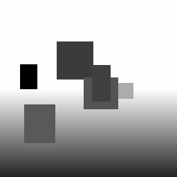
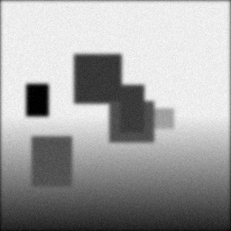
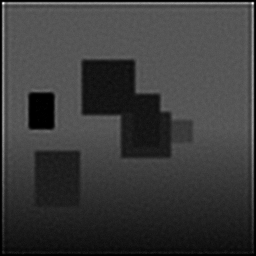
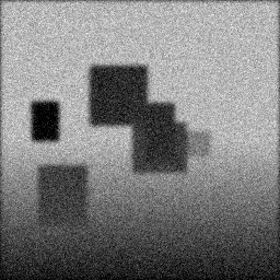
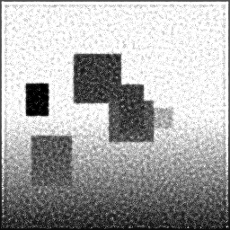
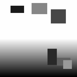
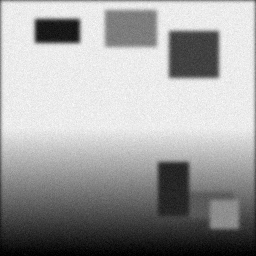
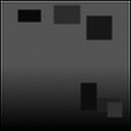
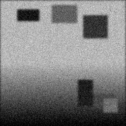
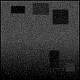
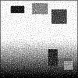
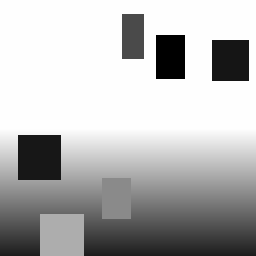
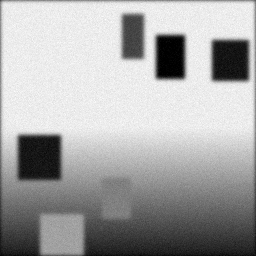
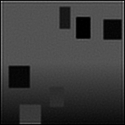
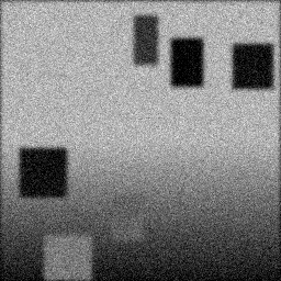
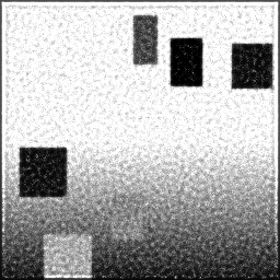
Reconstruction Gallery — 4 Scenes × 3 Scenarios
Method: CPU_baseline | Mismatch: nominal (nominal=True, perturbed=False)

Ground Truth
Measurement

Reconstruction
Ground Truth
Measurement
Reconstruction
Ground Truth
Measurement (perturbed)
Reconstruction


Mean PSNR Across All Scenes
Per-scene PSNR breakdown (4 scenes)
| Scene | I (PSNR) | I (SSIM) | II (PSNR) | II (SSIM) | III (PSNR) | III (SSIM) |
|---|---|---|---|---|---|---|
| scene_00 | 12.799733925471529 | 0.37968694072380205 | 12.071703569312016 | 0.35825143695994066 | 13.506763507797896 | 0.4021573644502054 |
| scene_01 | 5.806026384875609 | 0.4796046249826327 | 6.030423203911414 | 0.19344004863131214 | 18.47044552189445 | 0.22669922821491817 |
| scene_02 | 5.6571772261462066 | 0.46600075432368365 | 5.076086325487175 | 0.20923461502441765 | 18.605513677538003 | 0.23724583293967508 |
| scene_03 | 5.389777474892018 | 0.468956853362985 | 5.2322280218118955 | 0.2040550582761015 | 18.40005847928955 | 0.2386520108290784 |
| Mean | 7.41317875284634 | 0.4485622933482758 | 7.102610280130625 | 0.24124528972294298 | 17.245695296629975 | 0.2761886091084692 |
Experimental Setup
Key References
- Geiger et al., 'Are we ready for autonomous driving? The KITTI vision benchmark suite', CVPR 2012
Canonical Datasets
- KITTI 3D object detection
- nuScenes (1000 driving scenes)
- Waymo Open Dataset
Spec DAG — Forward Model Pipeline
P(pulsed) → Σ(return) → D(g, η₁)
Mismatch Parameters
| Symbol | Parameter | Description | Nominal | Perturbed |
|---|---|---|---|---|
| Δt | timing_jitter | Timing jitter (ps) | 0 | 50 |
| Δθ | beam_divergence | Beam divergence error (mrad) | 0 | 0.1 |
| ΔR | range_walk | Range walk error (cm) | 0 | 1.0 |
Credits System
Spec Primitives Reference (11 primitives)
Free-space or medium propagation kernel (Fresnel, Rayleigh-Sommerfeld).
Spatial or spatio-temporal amplitude modulation (coded aperture, SLM pattern).
Geometric projection operator (Radon transform, fan-beam, cone-beam).
Sampling in the Fourier / k-space domain (MRI, ptychography).
Shift-invariant convolution with a point-spread function (PSF).
Summation along a physical dimension (spectral, temporal, angular).
Sensor readout with gain g and noise model η (Gaussian, Poisson, mixed).
Patterned illumination (block, Hadamard, random) applied to the scene.
Spectral dispersion element (prism, grating) with shift α and aperture a.
Sample or gantry rotation (CT, electron tomography).
Spectral filter or monochromator selecting a wavelength band.