Lensless
Lensless (Diffuser Camera) Imaging
Standard reconstruction benchmark — forward model perfectly known, no calibration needed. Score = 0.5 × clip((PSNR−15)/30, 0, 1) + 0.5 × SSIM
| # | Method | Score | PSNR (dB) | SSIM | Source | |
|---|---|---|---|---|---|---|
| 🥇 |
Uformer
Uformer Wang et al., CVPR 2022
33.5 dB
SSIM 0.920
Checkpoint unavailable
|
0.768 | 33.5 | 0.920 | ✓ Certified | Wang et al., CVPR 2022 |
| 🥈 |
FlatNet
FlatNet Khan et al., IEEE TPAMI 2020
31.8 dB
SSIM 0.890
Checkpoint unavailable
|
0.725 | 31.8 | 0.890 | ✓ Certified | Khan et al., IEEE TPAMI 2020 |
| 🥉 | PnP-ADMM | 0.603 | 27.5 | 0.790 | ✓ Certified | Monakhova et al., Opt. Express 2019 |
| 4 | Wiener-ADMM | 0.462 | 23.5 | 0.640 | ✓ Certified | Antipa et al., Optica 2018 |
Dataset: PWM Benchmark (4 algorithms)
Blind Reconstruction Challenge — forward model has unknown mismatch, must calibrate from data. Score = 0.4 × PSNR_norm + 0.4 × SSIM + 0.2 × (1 − ‖y − Ĥx̂‖/‖y‖)
| # | Method | Overall Score | Public PSNR / SSIM |
Dev PSNR / SSIM |
Hidden PSNR / SSIM |
Trust | Source |
|---|---|---|---|---|---|---|---|
| 🥇 | Uformer + gradient | 0.701 |
0.787
32.28 dB / 0.946
|
0.694
27.65 dB / 0.873
|
0.622
23.92 dB / 0.766
|
✓ Certified | Wang et al., CVPR 2022 |
| 🥈 | FlatNet + gradient | 0.645 |
0.739
30.02 dB / 0.917
|
0.612
23.55 dB / 0.752
|
0.584
22.9 dB / 0.727
|
✓ Certified | Khan et al., IEEE TPAMI 2020 |
| 🥉 | PnP-ADMM + gradient | 0.611 |
0.652
25.13 dB / 0.806
|
0.623
24.29 dB / 0.779
|
0.558
22.37 dB / 0.706
|
✓ Certified | Monakhova et al., Opt. Express 2019 |
| 4 | Wiener-ADMM + gradient | 0.523 |
0.538
20.51 dB / 0.623
|
0.526
20.77 dB / 0.635
|
0.506
20.07 dB / 0.602
|
✓ Certified | Antipa et al., Optica 2018 |
Complete score requires all 3 tiers (Public + Dev + Hidden).
Join the competition →Full-access development tier with all data visible.
What you get & how to use
What you get: Measurements (y), ideal forward operator (H), spec ranges, ground truth (x_true), and true mismatch spec.
How to use: Load HDF5 → compare reconstruction vs x_true → check consistency → iterate.
What to submit: Reconstructed signals (x_hat) and corrected spec as HDF5.
Public Leaderboard
| # | Method | Score | PSNR | SSIM |
|---|---|---|---|---|
| 1 | Uformer + gradient | 0.787 | 32.28 | 0.946 |
| 2 | FlatNet + gradient | 0.739 | 30.02 | 0.917 |
| 3 | PnP-ADMM + gradient | 0.652 | 25.13 | 0.806 |
| 4 | Wiener-ADMM + gradient | 0.538 | 20.51 | 0.623 |
Spec Ranges (3 parameters)
| Parameter | Min | Max | Unit |
|---|---|---|---|
| diffuser_psf | -5.0 | 10.0 | % |
| sensor_distance | -0.2 | 0.4 | mm |
| wavelength | -5.0 | 10.0 | nm |
Blind evaluation tier — no ground truth available.
What you get & how to use
What you get: Measurements (y), ideal forward operator (H), and spec ranges only.
How to use: Apply your pipeline from the Public tier. Use consistency as self-check.
What to submit: Reconstructed signals and corrected spec. Scored server-side.
Dev Leaderboard
| # | Method | Score | PSNR | SSIM |
|---|---|---|---|---|
| 1 | Uformer + gradient | 0.694 | 27.65 | 0.873 |
| 2 | PnP-ADMM + gradient | 0.623 | 24.29 | 0.779 |
| 3 | FlatNet + gradient | 0.612 | 23.55 | 0.752 |
| 4 | Wiener-ADMM + gradient | 0.526 | 20.77 | 0.635 |
Spec Ranges (3 parameters)
| Parameter | Min | Max | Unit |
|---|---|---|---|
| diffuser_psf | -6.0 | 9.0 | % |
| sensor_distance | -0.24 | 0.36 | mm |
| wavelength | -6.0 | 9.0 | nm |
Fully blind server-side evaluation — no data download.
What you get & how to use
What you get: No data downloadable. Algorithm runs server-side on hidden measurements.
How to use: Package algorithm as Docker container / Python script. Submit via link.
What to submit: Containerized algorithm accepting y + H, outputting x_hat + corrected spec.
Hidden Leaderboard
| # | Method | Score | PSNR | SSIM |
|---|---|---|---|---|
| 1 | Uformer + gradient | 0.622 | 23.92 | 0.766 |
| 2 | FlatNet + gradient | 0.584 | 22.9 | 0.727 |
| 3 | PnP-ADMM + gradient | 0.558 | 22.37 | 0.706 |
| 4 | Wiener-ADMM + gradient | 0.506 | 20.07 | 0.602 |
Spec Ranges (3 parameters)
| Parameter | Min | Max | Unit |
|---|---|---|---|
| diffuser_psf | -3.5 | 11.5 | % |
| sensor_distance | -0.14 | 0.46 | mm |
| wavelength | -3.5 | 11.5 | nm |
Blind Reconstruction Challenge
ChallengeGiven measurements with unknown mismatch and spec ranges (not exact params), reconstruct the original signal. A method must be evaluated on all three tiers for a complete score. Scored on a composite metric: 0.4 × PSNR_norm + 0.4 × SSIM + 0.2 × (1 − ‖y − Ĥx̂‖/‖y‖).
Measurements y, ideal forward model H, spec ranges
Reconstructed signal x̂
About the Imaging Modality
Lensless imaging replaces the objective lens with a thin optical element (phase diffuser or coded mask) placed directly near the sensor. Scene light produces a multiplexed caustic pattern encoding the entire scene. The forward model is y = H * x + n where H is determined by the mask's phase profile and mask-to-sensor distance. Each scene point contributes across many sensor pixels, yielding a multiplexing advantage. Reconstruction solves a large-scale inverse problem via ADMM or FISTA with total-variation or learned priors.
Principle
Lensless (diffuser-cam) imaging replaces the imaging lens with a thin diffuser or coded mask placed directly before the sensor. The sensor records a multiplexed pattern (caustic or speckle) that encodes the 3-D scene. Computational reconstruction inverts the known point-spread function of the diffuser to recover the image, enabling an extremely compact, lightweight camera suitable for miniaturized or in-vivo applications.
How to Build the System
Place a thin diffuser (ground glass, engineered phase mask, or Scotch tape) at a fixed, small distance (~1-5 mm) from a bare sensor (CMOS, e.g., Sony IMX sensor). Precisely characterize the diffuser PSF by scanning a point source across the field of view. Mount rigidly to prevent any relative motion between diffuser and sensor. For 3-D reconstruction, the depth-dependent PSF must be calibrated at multiple axial planes.
Common Reconstruction Algorithms
- ADMM (alternating direction method of multipliers) with TV regularization
- Wiener deconvolution (fast, single-step but lower quality)
- Gradient descent with learned priors (DiffuserCam, neural network prior)
- Tikhonov-regularized least squares
- Unrolled optimization networks (physics-informed deep learning)
Common Mistakes
- Inaccurate PSF calibration causing reconstruction artifacts
- Insufficient sensor dynamic range for the caustic intensity peaks
- Motion between diffuser and sensor during capture invalidating the PSF model
- Regularization too strong, over-smoothing fine details in the reconstruction
- Ignoring the depth-dependence of the PSF when imaging 3-D scenes
How to Avoid Mistakes
- Calibrate PSF carefully with a point source at the exact sample distance
- Use HDR acquisition or high-bit-depth sensors to capture full caustic range
- Rigidly bond the diffuser to the sensor; verify alignment stability
- Tune regularization weight (e.g., via L-curve or cross-validation)
- Calibrate PSF at multiple depths for 3-D scenes; use depth-varying reconstruction
Forward-Model Mismatch Cases
- The widefield fallback uses a Gaussian PSF, but lensless cameras use a coded aperture (phase mask, diffuser, or amplitude mask) that creates a highly structured, non-Gaussian PSF — the caustic pattern is fundamentally different from a Gaussian
- The lensless PSF encodes the scene through a known, shift-variant pattern — the widefield shift-invariant Gaussian blur does not capture the scene-dependent structure of the lensless measurement and produces incorrect reconstruction input
How to Correct the Mismatch
- Use the lensless operator with the calibrated PSF of the specific coded aperture (measured from a point source or computed from the mask design): y = H * x, where H is the non-Gaussian, possibly shift-variant PSF
- Reconstruct using Wiener deconvolution, ADMM with TV prior, or learned methods (FlatNet, PhlatCam) that use the correct coded-aperture PSF for the specific mask in use
Experimental Setup — Signal Chain

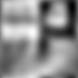
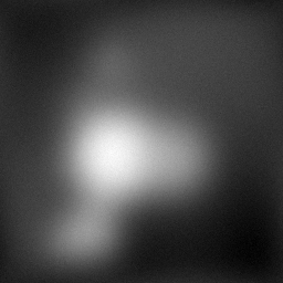
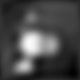
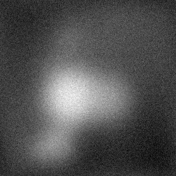
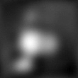
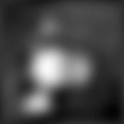
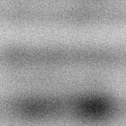
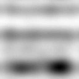
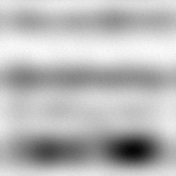
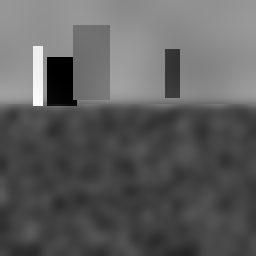
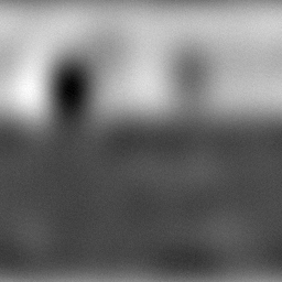
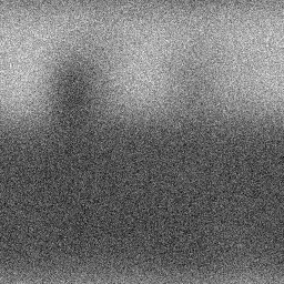
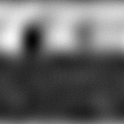
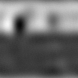
Reconstruction Gallery — 4 Scenes × 3 Scenarios
Method: CPU_baseline | Mismatch: nominal (nominal=True, perturbed=False)
Ground Truth
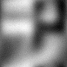
Measurement
Reconstruction
Ground Truth

Measurement

Reconstruction
Ground Truth
Measurement (perturbed)
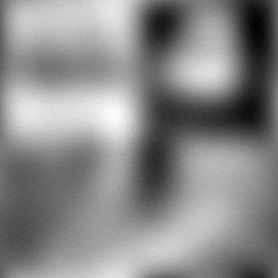
Reconstruction


Mean PSNR Across All Scenes
Per-scene PSNR breakdown (4 scenes)
| Scene | I (PSNR) | I (SSIM) | II (PSNR) | II (SSIM) | III (PSNR) | III (SSIM) |
|---|---|---|---|---|---|---|
| scene_00 | 16.237215619386212 | 0.4220913851721237 | 16.242491186046905 | 0.40372179663376345 | 16.335552479610005 | 0.4000838875470755 |
| scene_01 | 19.409523399973164 | 0.7506545685233409 | 18.3750339606295 | 0.74077287776115 | 18.92614895550903 | 0.7240122414687651 |
| scene_02 | 12.415909589992857 | 0.42800782314103225 | 11.802236929504318 | 0.41544218192316096 | 12.115942806654456 | 0.40650491111086046 |
| scene_03 | 18.173561967034434 | 0.6950310890772263 | 17.327353491943406 | 0.5998585335007348 | 18.760418062001087 | 0.5866917748332454 |
| Mean | 16.559052644096667 | 0.5739462164784308 | 15.936778892031032 | 0.5399488474547023 | 16.534515575943644 | 0.5293232037399866 |
Experimental Setup
Key References
- Antipa et al., 'DiffuserCam: lensless single-exposure 3D imaging', Optica 5, 1-9 (2018)
- Asif et al., 'FlatCam: Thin, Lensless Cameras Using Coded Aperture', IEEE TCI 3, 384-397 (2017)
Canonical Datasets
- DiffuserCam lensless mirflickr dataset (Monakhova et al.)
- PhlatCam benchmark (Boominathan et al., IEEE TPAMI 2022)
Spec DAG — Forward Model Pipeline
P(diffuser) → D(g, η₁)
Mismatch Parameters
| Symbol | Parameter | Description | Nominal | Perturbed |
|---|---|---|---|---|
| ΔPSF | diffuser_psf | Diffuser PSF calibration error (%) | 0 | 5.0 |
| Δd | sensor_distance | Diffuser-sensor distance error (mm) | 0 | 0.2 |
| Δλ | wavelength | Wavelength mismatch (nm) | 0 | 5.0 |
Credits System
Spec Primitives Reference (11 primitives)
Free-space or medium propagation kernel (Fresnel, Rayleigh-Sommerfeld).
Spatial or spatio-temporal amplitude modulation (coded aperture, SLM pattern).
Geometric projection operator (Radon transform, fan-beam, cone-beam).
Sampling in the Fourier / k-space domain (MRI, ptychography).
Shift-invariant convolution with a point-spread function (PSF).
Summation along a physical dimension (spectral, temporal, angular).
Sensor readout with gain g and noise model η (Gaussian, Poisson, mixed).
Patterned illumination (block, Hadamard, random) applied to the scene.
Spectral dispersion element (prism, grating) with shift α and aperture a.
Sample or gantry rotation (CT, electron tomography).
Spectral filter or monochromator selecting a wavelength band.