Integral
Integral Photography
Standard reconstruction benchmark — forward model perfectly known, no calibration needed. Score = 0.5 × clip((PSNR−15)/30, 0, 1) + 0.5 × SSIM
| # | Method | Score | PSNR (dB) | SSIM | Source | |
|---|---|---|---|---|---|---|
| 🥇 |
DistgSSR
DistgSSR Wang et al., CVPR 2022
35.8 dB
SSIM 0.950
Checkpoint unavailable
|
0.822 | 35.8 | 0.950 | ✓ Certified | Wang et al., CVPR 2022 |
| 🥈 |
LFAttNet
LFAttNet Tsai et al., IEEE TIP 2020
33.5 dB
SSIM 0.920
Checkpoint unavailable
|
0.768 | 33.5 | 0.920 | ✓ Certified | Tsai et al., IEEE TIP 2020 |
| 🥉 | PnP-LF | 0.648 | 29.0 | 0.830 | ✓ Certified | PnP-ADMM with LF prior |
| 4 | Shift-and-Add | 0.517 | 25.0 | 0.700 | ✓ Certified | Ng et al., Stanford Tech Report 2005 |
Dataset: PWM Benchmark (4 algorithms)
Blind Reconstruction Challenge — forward model has unknown mismatch, must calibrate from data. Score = 0.4 × PSNR_norm + 0.4 × SSIM + 0.2 × (1 − ‖y − Ĥx̂‖/‖y‖)
| # | Method | Overall Score | Public PSNR / SSIM |
Dev PSNR / SSIM |
Hidden PSNR / SSIM |
Trust | Source |
|---|---|---|---|---|---|---|---|
| 🥇 | DistgSSR + gradient | 0.741 |
0.816
34.13 dB / 0.962
|
0.728
29.22 dB / 0.904
|
0.678
27.66 dB / 0.873
|
✓ Certified | Wang et al., CVPR 2022 |
| 🥈 | LFAttNet + gradient | 0.679 |
0.764
31.65 dB / 0.939
|
0.671
26.59 dB / 0.848
|
0.602
23.3 dB / 0.743
|
✓ Certified | Tsai et al., IEEE TIP 2020 |
| 🥉 | PnP-LF + gradient | 0.663 |
0.713
27.73 dB / 0.875
|
0.641
24.64 dB / 0.791
|
0.635
24.94 dB / 0.800
|
✓ Certified | PnP-ADMM with LF prior |
| 4 | Shift-and-Add + gradient | 0.534 |
0.584
22.32 dB / 0.703
|
0.543
20.89 dB / 0.641
|
0.476
18.88 dB / 0.544
|
✓ Certified | Ng et al., Stanford Tech Report 2005 |
Complete score requires all 3 tiers (Public + Dev + Hidden).
Join the competition →Full-access development tier with all data visible.
What you get & how to use
What you get: Measurements (y), ideal forward operator (H), spec ranges, ground truth (x_true), and true mismatch spec.
How to use: Load HDF5 → compare reconstruction vs x_true → check consistency → iterate.
What to submit: Reconstructed signals (x_hat) and corrected spec as HDF5.
Public Leaderboard
| # | Method | Score | PSNR | SSIM |
|---|---|---|---|---|
| 1 | DistgSSR + gradient | 0.816 | 34.13 | 0.962 |
| 2 | LFAttNet + gradient | 0.764 | 31.65 | 0.939 |
| 3 | PnP-LF + gradient | 0.713 | 27.73 | 0.875 |
| 4 | Shift-and-Add + gradient | 0.584 | 22.32 | 0.703 |
Spec Ranges (3 parameters)
| Parameter | Min | Max | Unit |
|---|---|---|---|
| lens_pitch | -1.0 | 2.0 | μm |
| gap_distance | -5.0 | 10.0 | μm |
| aberration | -0.1 | 0.2 | waves |
Blind evaluation tier — no ground truth available.
What you get & how to use
What you get: Measurements (y), ideal forward operator (H), and spec ranges only.
How to use: Apply your pipeline from the Public tier. Use consistency as self-check.
What to submit: Reconstructed signals and corrected spec. Scored server-side.
Dev Leaderboard
| # | Method | Score | PSNR | SSIM |
|---|---|---|---|---|
| 1 | DistgSSR + gradient | 0.728 | 29.22 | 0.904 |
| 2 | LFAttNet + gradient | 0.671 | 26.59 | 0.848 |
| 3 | PnP-LF + gradient | 0.641 | 24.64 | 0.791 |
| 4 | Shift-and-Add + gradient | 0.543 | 20.89 | 0.641 |
Spec Ranges (3 parameters)
| Parameter | Min | Max | Unit |
|---|---|---|---|
| lens_pitch | -1.2 | 1.8 | μm |
| gap_distance | -6.0 | 9.0 | μm |
| aberration | -0.12 | 0.18 | waves |
Fully blind server-side evaluation — no data download.
What you get & how to use
What you get: No data downloadable. Algorithm runs server-side on hidden measurements.
How to use: Package algorithm as Docker container / Python script. Submit via link.
What to submit: Containerized algorithm accepting y + H, outputting x_hat + corrected spec.
Hidden Leaderboard
| # | Method | Score | PSNR | SSIM |
|---|---|---|---|---|
| 1 | DistgSSR + gradient | 0.678 | 27.66 | 0.873 |
| 2 | PnP-LF + gradient | 0.635 | 24.94 | 0.8 |
| 3 | LFAttNet + gradient | 0.602 | 23.3 | 0.743 |
| 4 | Shift-and-Add + gradient | 0.476 | 18.88 | 0.544 |
Spec Ranges (3 parameters)
| Parameter | Min | Max | Unit |
|---|---|---|---|
| lens_pitch | -0.7 | 2.3 | μm |
| gap_distance | -3.5 | 11.5 | μm |
| aberration | -0.07 | 0.23 | waves |
Blind Reconstruction Challenge
ChallengeGiven measurements with unknown mismatch and spec ranges (not exact params), reconstruct the original signal. A method must be evaluated on all three tiers for a complete score. Scored on a composite metric: 0.4 × PSNR_norm + 0.4 × SSIM + 0.2 × (1 − ‖y − Ĥx̂‖/‖y‖).
Measurements y, ideal forward model H, spec ranges
Reconstructed signal x̂
About the Imaging Modality
Integral photography (IP), originally proposed by Lippmann in 1908, captures a light field using a fly-eye lens array (matrix of small lenses) where each lenslet records a small elemental image from a slightly different perspective. The array of elemental images encodes 3D scene information, enabling computational refocusing, depth estimation, and autostereoscopic 3D display. Compared to microlens-based plenoptic cameras, IP typically uses larger lenslets with correspondingly more pixels per lens. Reconstruction includes depth-from-correspondence between elemental images and 3D focal stack computation.
Principle
Integral photography (also known as integral imaging) uses a 2-D array of elemental lenses to capture multi-perspective views of a 3-D scene simultaneously. Each elemental lens records a small perspective image, and the full set encodes the 4-D light field. Computational reconstruction produces 3-D images that can be viewed from different angles or refocused without glasses.
How to Build the System
Place a 2-D microlens or lenslet array (pitch 0.5-1 mm, ~50-200 elements per side) at one focal length from a high-resolution sensor. Each lenslet forms a separate elemental image. For display: show the integral image on a high-resolution display with a matched output lenslet array. Calibrate lenslet grid alignment, individual lens focal lengths, and vignetting correction. Use telecentric imaging for uniform magnification.
Common Reconstruction Algorithms
- Computational refocusing via pixel rearrangement and summation
- Depth estimation from elemental image disparity analysis
- 3-D scene reconstruction from integral images
- Super-resolution integral imaging (combining multiple shifted captures)
- Deep-learning integral image reconstruction and view synthesis
Common Mistakes
- Lenslet array not properly aligned with the sensor pixel grid
- Insufficient number of elemental lenses for the desired depth range
- Crosstalk between adjacent elemental images due to lens aberrations
- Not correcting for vignetting variations across the lenslet array
- Pseudoscopic (depth-reversed) images if reconstruction is not properly handled
How to Avoid Mistakes
- Align lenslet array to sensor with precision jigs and verify with calibration patterns
- Design lenslet pitch and focal length for the required depth-of-field
- Use high-quality molded lenslets and baffles to minimize crosstalk
- Apply per-lenslet calibration including vignetting and distortion correction
- Use computational depth inversion to correct pseudoscopic effects
Forward-Model Mismatch Cases
- The widefield fallback produces a single-perspective blurred image, but integral imaging captures multiple sub-aperture views through a lenslet array — each elemental image sees the scene from a slightly different angle
- Without the lenslet-array angular encoding, depth information (parallax between views) is lost — computational refocusing and 3D reconstruction from the fallback output are impossible
How to Correct the Mismatch
- Use the integral imaging operator that models the lenslet array: each microlens captures a different angular perspective, encoding the 4D light field on the 2D sensor
- Reconstruct depth maps via disparity estimation between elemental images, and perform computational refocusing using pixel rearrangement and summation across sub-aperture views
Experimental Setup — Signal Chain

Reconstruction Gallery — 4 Scenes × 3 Scenarios
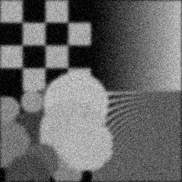
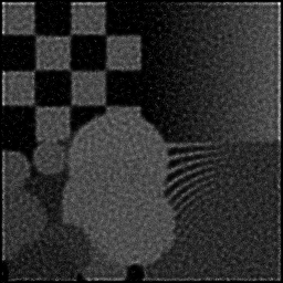
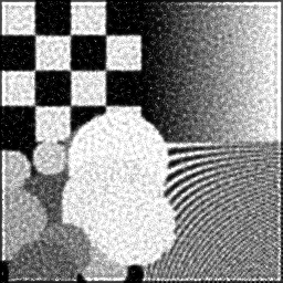
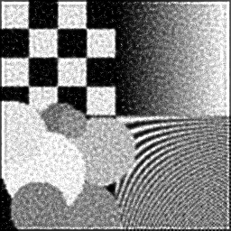
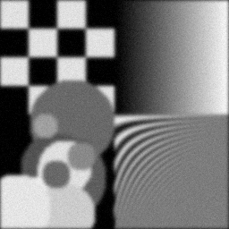
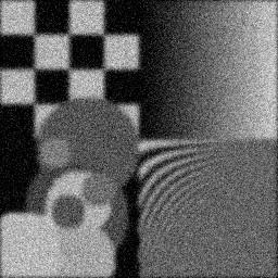
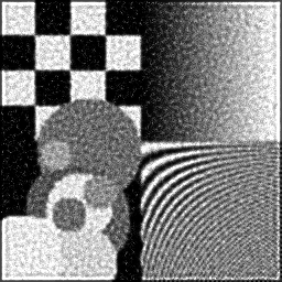
Method: CPU_baseline | Mismatch: nominal (nominal=True, perturbed=False)

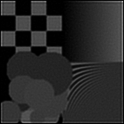
Ground Truth
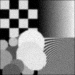
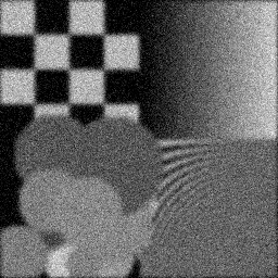
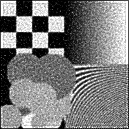
Measurement
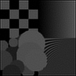
Reconstruction
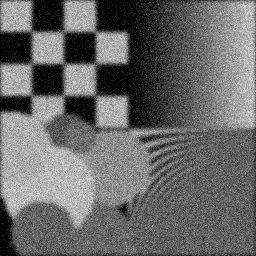
Ground Truth
Measurement
Reconstruction
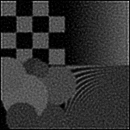
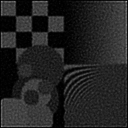
Ground Truth
Measurement (perturbed)
Reconstruction


Mean PSNR Across All Scenes
Per-scene PSNR breakdown (4 scenes)
| Scene | I (PSNR) | I (SSIM) | II (PSNR) | II (SSIM) | III (PSNR) | III (SSIM) |
|---|---|---|---|---|---|---|
| scene_00 | 6.831755145049858 | 0.39251757962307293 | 6.747744781788927 | 0.19624154301519284 | 17.0733092814934 | 0.34599733923876136 |
| scene_01 | 7.208081904434112 | 0.39392374023822935 | 7.395701051446139 | 0.19865145380844743 | 16.91778445629049 | 0.35342995245672976 |
| scene_02 | 7.675436503843393 | 0.39375468365060645 | 7.1143972480104045 | 0.20103810356474872 | 16.88449427499023 | 0.37603178319129643 |
| scene_03 | 7.8398378914912294 | 0.39507824343020287 | 7.670146776544666 | 0.1976384681380463 | 16.96130682502457 | 0.341813373374832 |
| Mean | 7.388777861204648 | 0.39381856173552793 | 7.231997464447534 | 0.1983923921316088 | 16.959223709449674 | 0.35431811206540487 |
Experimental Setup
Key References
- Lippmann, C. R. Acad. Sci. Paris 146, 446 (1908)
- Park et al., 'Recent progress in 3D imaging systems', J. Opt. Soc. Am. A 26, 2538 (2009)
Canonical Datasets
- ETRI integral imaging test set
- Middlebury multi-view stereo (adapted)
Spec DAG — Forward Model Pipeline
Π(lens-array) → D(g, η₁)
Mismatch Parameters
| Symbol | Parameter | Description | Nominal | Perturbed |
|---|---|---|---|---|
| Δp | lens_pitch | Lens pitch error (μm) | 0 | 1.0 |
| Δd | gap_distance | Lens-to-sensor gap error (μm) | 0 | 5.0 |
| ΔW | aberration | Lens aberration (waves) | 0 | 0.1 |
Credits System
Spec Primitives Reference (11 primitives)
Free-space or medium propagation kernel (Fresnel, Rayleigh-Sommerfeld).
Spatial or spatio-temporal amplitude modulation (coded aperture, SLM pattern).
Geometric projection operator (Radon transform, fan-beam, cone-beam).
Sampling in the Fourier / k-space domain (MRI, ptychography).
Shift-invariant convolution with a point-spread function (PSF).
Summation along a physical dimension (spectral, temporal, angular).
Sensor readout with gain g and noise model η (Gaussian, Poisson, mixed).
Patterned illumination (block, Hadamard, random) applied to the scene.
Spectral dispersion element (prism, grating) with shift α and aperture a.
Sample or gantry rotation (CT, electron tomography).
Spectral filter or monochromator selecting a wavelength band.