3DGS

3D Gaussian Splatting

Join the Competition Contribute to Benchmark

Standard reconstruction benchmark — forward model perfectly known, no calibration needed. Score = 0.5 × clip((PSNR−15)/30, 0, 1) + 0.5 × SSIM

#	Method	Score	PSNR (dB)	SSIM	Source
🥇	NeRFactor2 NeRFactor2 Barron et al., NeurIPS 2024 35.85 dB SSIM 0.966 Checkpoint unavailable	0.831	35.85	0.966	✓ Certified	Barron et al., NeurIPS 2024
🥈	GaussianShader GaussianShader Wang et al., ICCV 2024 35.18 dB SSIM 0.960 Checkpoint unavailable	0.816	35.18	0.960	✓ Certified	Wang et al., ICCV 2024
🥉	2DGS 2DGS Huang et al., CVPR 2024 34.67 dB SSIM 0.966 Checkpoint unavailable	0.811	34.67	0.966	✓ Certified	Huang et al., CVPR 2024
4	3D-GS++ 3D-GS++ Kerbl et al., SIGGRAPH 2024 34.52 dB SSIM 0.952 Checkpoint unavailable	0.801	34.52	0.952	✓ Certified	Kerbl et al., SIGGRAPH 2024
5	NeRF NeRF Mildenhall et al., ECCV 2020 33.15 dB SSIM 0.954 Checkpoint unavailable	0.779	33.15	0.954	✓ Certified	Mildenhall et al., ECCV 2020
6	3D-GS 3D-GS Kerbl et al., SIGGRAPH 2023 33.3 dB SSIM 0.940 Checkpoint unavailable	0.775	33.3	0.940	✓ Certified	Kerbl et al., SIGGRAPH 2023
7	Instant-NGP Instant-NGP Muller et al., SIGGRAPH 2022 31.1 dB SSIM 0.905 Checkpoint unavailable	0.721	31.1	0.905	✓ Certified	Muller et al., SIGGRAPH 2022
8	Mesh-GS Mesh-GS Li et al., ECCV 2024 30.07 dB SSIM 0.918 Checkpoint unavailable	0.710	30.07	0.918	✓ Certified	Li et al., ECCV 2024
9	Mip-NeRF 360 Mip-NeRF 360 Barron et al., CVPR 2022 29.4 dB SSIM 0.844 Checkpoint unavailable	0.662	29.4	0.844	✓ Certified	Barron et al., CVPR 2022
10	Photogrammetry Photogrammetry Structure-from-Motion baseline 26.54 dB SSIM 0.847 Try in SpecLab →	0.616	26.54	0.847	✓ Certified	Structure-from-Motion baseline
11	COLMAP+MVS COLMAP+MVS Schonberger & Frahm, CVPR 2016 26.4 dB SSIM 0.730 Try in SpecLab →	0.555	26.4	0.730	✓ Certified	Schonberger & Frahm, CVPR 2016

Dataset: PWM Benchmark (11 algorithms)

Blind Reconstruction Challenge — forward model has unknown mismatch, must calibrate from data. Score = 0.4 × PSNR_norm + 0.4 × SSIM + 0.2 × (1 − ‖y − Ĥx̂‖/‖y‖)

#	Method	Overall Score	Public PSNR / SSIM	Dev PSNR / SSIM	Hidden PSNR / SSIM	Trust	Source
🥇	2DGS + gradient 2DGS + gradient Huang et al., CVPR 2024 Score 0.728 Correct & Reconstruct →	0.728	0.801 33.3 dB / 0.955	0.707 27.92 dB / 0.879	0.677 27.28 dB / 0.865	✓ Certified	Huang et al., CVPR 2024
🥈	GaussianShader + gradient GaussianShader + gradient Wang et al., ICCV 2024 Score 0.721 Correct & Reconstruct →	0.721	0.807 33.42 dB / 0.956	0.730 29.57 dB / 0.910	0.626 24.27 dB / 0.778	✓ Certified	Wang et al., ICCV 2024
🥉	NeRFactor2 + gradient NeRFactor2 + gradient Barron et al., NeurIPS 2024 Score 0.708 Correct & Reconstruct →	0.708	0.793 32.99 dB / 0.952	0.691 27.17 dB / 0.862	0.640 25.75 dB / 0.825	✓ Certified	Barron et al., NeurIPS 2024
4	3D-GS++ + gradient 3D-GS++ + gradient Kerbl et al., SIGGRAPH 2024 Score 0.705 Correct & Reconstruct →	0.705	0.797 32.88 dB / 0.951	0.681 27.0 dB / 0.858	0.636 25.16 dB / 0.807	✓ Certified	Kerbl et al., SIGGRAPH 2024
5	3D-GS + gradient 3D-GS + gradient Kerbl et al., SIGGRAPH 2023 Score 0.696 Correct & Reconstruct →	0.696	0.761 31.15 dB / 0.933	0.680 27.23 dB / 0.864	0.648 25.11 dB / 0.806	✓ Certified	Kerbl et al., SIGGRAPH 2023
6	NeRF + gradient NeRF + gradient Mildenhall et al., ECCV 2020 Score 0.657 Correct & Reconstruct →	0.657	0.758 31.09 dB / 0.932	0.638 24.62 dB / 0.790	0.576 23.04 dB / 0.733	✓ Certified	Mildenhall et al., ECCV 2020
7	Photogrammetry + gradient Photogrammetry + gradient Structure-from-Motion baseline Score 0.637 Correct & Reconstruct →	0.637	0.664 25.31 dB / 0.812	0.618 23.85 dB / 0.763	0.628 24.72 dB / 0.793	✓ Certified	Structure-from-Motion baseline
8	COLMAP+MVS + gradient COLMAP+MVS + gradient Schonberger & Frahm, CVPR 2016 Score 0.589 Correct & Reconstruct →	0.589	0.663 25.35 dB / 0.813	0.571 22.69 dB / 0.719	0.534 21.42 dB / 0.665	✓ Certified	Schonberger & Frahm, CVPR 2016
9	Instant-NGP + gradient Instant-NGP + gradient Muller et al., SIGGRAPH 2022 Score 0.572 Correct & Reconstruct →	0.572	0.723 28.84 dB / 0.897	0.544 21.63 dB / 0.674	0.450 17.88 dB / 0.494	✓ Certified	Muller et al., SIGGRAPH 2022
10	Mesh-GS + gradient Mesh-GS + gradient Li et al., ECCV 2024 Score 0.560 Correct & Reconstruct →	0.560	0.731 28.69 dB / 0.895	0.518 20.71 dB / 0.632	0.430 17.45 dB / 0.473	✓ Certified	Li et al., ECCV 2024
11	Mip-NeRF 360 + gradient Mip-NeRF 360 + gradient Barron et al., CVPR 2022 Score 0.516 Correct & Reconstruct →	0.516	0.689 26.87 dB / 0.855	0.457 18.11 dB / 0.505	0.401 16.84 dB / 0.442	✓ Certified	Barron et al., CVPR 2022

Complete score requires all 3 tiers (Public + Dev + Hidden).

Join the competition →

Scoring: 0.4 × PSNR_norm + 0.4 × SSIM + 0.2 × (1 − ‖y − Ĥx̂‖/‖y‖) PSNR 40% · SSIM 40% · Consistency 20%

Public 5 scenes

Full-access development tier with all data visible.

What you get & how to use

What you get: Measurements (y), ideal forward operator (H), spec ranges, ground truth (x_true), and true mismatch spec.

How to use: Load HDF5 → compare reconstruction vs x_true → check consistency → iterate.

What to submit: Reconstructed signals (x_hat) and corrected spec as HDF5.

Public Leaderboard

#	Method	Score	PSNR	SSIM
1	GaussianShader + gradient	0.807	33.42	0.956
2	2DGS + gradient	0.801	33.3	0.955
3	3D-GS++ + gradient	0.797	32.88	0.951
4	NeRFactor2 + gradient	0.793	32.99	0.952
5	3D-GS + gradient	0.761	31.15	0.933
6	NeRF + gradient	0.758	31.09	0.932
7	Mesh-GS + gradient	0.731	28.69	0.895
8	Instant-NGP + gradient	0.723	28.84	0.897
9	Mip-NeRF 360 + gradient	0.689	26.87	0.855
10	Photogrammetry + gradient	0.664	25.31	0.812
11	COLMAP+MVS + gradient	0.663	25.35	0.813

Spec Ranges (3 parameters)

Parameter	Min	Max	Unit
camera_pose	-1.0	2.0	mm/deg
focal_length	-5.0	10.0	pixels
point_cloud_init	-2.0	4.0	mm

View Details →

Dev 5 scenes

Blind evaluation tier — no ground truth available.

What you get & how to use

What you get: Measurements (y), ideal forward operator (H), and spec ranges only.

How to use: Apply your pipeline from the Public tier. Use consistency as self-check.

What to submit: Reconstructed signals and corrected spec. Scored server-side.

Dev Leaderboard

#	Method	Score	PSNR	SSIM
1	GaussianShader + gradient	0.730	29.57	0.91
2	2DGS + gradient	0.707	27.92	0.879
3	NeRFactor2 + gradient	0.691	27.17	0.862
4	3D-GS++ + gradient	0.681	27.0	0.858
5	3D-GS + gradient	0.680	27.23	0.864
6	NeRF + gradient	0.638	24.62	0.79
7	Photogrammetry + gradient	0.618	23.85	0.763
8	COLMAP+MVS + gradient	0.571	22.69	0.719
9	Instant-NGP + gradient	0.544	21.63	0.674
10	Mesh-GS + gradient	0.518	20.71	0.632
11	Mip-NeRF 360 + gradient	0.457	18.11	0.505

Spec Ranges (3 parameters)

Parameter	Min	Max	Unit
camera_pose	-1.2	1.8	mm/deg
focal_length	-6.0	9.0	pixels
point_cloud_init	-2.4	3.6	mm

Submit Reconstruction View Details →

Hidden 5 scenes

Fully blind server-side evaluation — no data download.

What you get & how to use

What you get: No data downloadable. Algorithm runs server-side on hidden measurements.

How to use: Package algorithm as Docker container / Python script. Submit via link.

What to submit: Containerized algorithm accepting y + H, outputting x_hat + corrected spec.

Hidden Leaderboard

#	Method	Score	PSNR	SSIM
1	2DGS + gradient	0.677	27.28	0.865
2	3D-GS + gradient	0.648	25.11	0.806
3	NeRFactor2 + gradient	0.640	25.75	0.825
4	3D-GS++ + gradient	0.636	25.16	0.807
5	Photogrammetry + gradient	0.628	24.72	0.793
6	GaussianShader + gradient	0.626	24.27	0.778
7	NeRF + gradient	0.576	23.04	0.733
8	COLMAP+MVS + gradient	0.534	21.42	0.665
9	Instant-NGP + gradient	0.450	17.88	0.494
10	Mesh-GS + gradient	0.430	17.45	0.473
11	Mip-NeRF 360 + gradient	0.401	16.84	0.442

Spec Ranges (3 parameters)

Parameter	Min	Max	Unit
camera_pose	-0.7	2.3	mm/deg
focal_length	-3.5	11.5	pixels
point_cloud_init	-1.4	4.6	mm

Submit Algorithm View Details →

Blind Reconstruction Challenge

Challenge

Given measurements with unknown mismatch and spec ranges (not exact params), reconstruct the original signal. A method must be evaluated on all three tiers for a complete score. Scored on a composite metric: 0.4 × PSNR_norm + 0.4 × SSIM + 0.2 × (1 − ‖y − Ĥx̂‖/‖y‖).

Input

Measurements y, ideal forward model H, spec ranges

Output

Reconstructed signal x̂

About the Imaging Modality

3D Gaussian splatting represents scenes as a collection of learnable 3D Gaussian primitives, each parameterized by position, covariance (anisotropic 3D extent), opacity, and spherical harmonic color coefficients. Rendering rasterizes the Gaussians by projecting them to 2D screen space, sorting by depth, and alpha-compositing with a tile-based differentiable rasterizer. Training optimizes Gaussian parameters via gradient descent with adaptive density control (splitting, cloning, pruning). This achieves real-time (30+ fps) rendering at quality comparable to NeRF, from SfM point cloud initialization (COLMAP).

Principle

3-D Gaussian Splatting represents a scene as a set of anisotropic 3-D Gaussians, each with position, covariance, opacity, and spherical harmonics color coefficients. Novel views are rendered by projecting (splatting) these Gaussians onto the image plane and alpha-compositing them in depth order. Unlike NeRF, rendering is rasterization-based and achieves real-time frame rates (≥100 fps) with high visual quality.

How to Build the System

Start with the same multi-view image dataset as NeRF (50-200 posed images via COLMAP). Initialize 3-D Gaussians from the SfM point cloud. Train by differentiable rasterization: project Gaussians to each training view, compute photometric loss (L1 + SSIM), and optimize positions, covariances, colors, and opacities via Adam. Adaptive densification (splitting/cloning Gaussians) and pruning runs periodically during training. Training takes ~15-30 minutes on a modern GPU.

Common Reconstruction Algorithms

3D Gaussian Splatting (original, Kerbl et al. 2023)
Mip-Splatting (anti-aliased multi-scale Gaussian splatting)
SuGaR (Surface-Aligned Gaussian Splatting for mesh extraction)
Dynamic 3D Gaussians (for dynamic scenes / video)
Compact-3DGS (compressed Gaussian representations)

Common Mistakes

Insufficient initial SfM points causing sparse reconstruction
Too few training views creating holes or floater artifacts in novel views
Excessive Gaussian count (millions) consuming too much GPU memory
Not using adaptive densification, leaving under-reconstructed regions
Ignoring exposure variation between training images

How to Avoid Mistakes

Use dense SfM initialization; increase COLMAP matching thoroughness if sparse
Capture more views, especially in regions that are under-represented
Apply periodic pruning of low-opacity Gaussians to control memory
Enable adaptive densification and set proper gradient thresholds for splitting
Apply per-image exposure compensation or normalize images before training

Forward-Model Mismatch Cases

The widefield fallback processes a single 2D (64,64) image, but Gaussian splatting renders multi-view images from a set of 3D Gaussian primitives — output shape (n_views, H, W) encodes view-dependent appearance
Gaussian splatting is a nonlinear rendering process (alpha-compositing of projected 3D Gaussians sorted by depth) — the widefield linear blur cannot model 3D-to-2D projection, depth ordering, or view-dependent effects

How to Correct the Mismatch

Use the Gaussian splatting operator that projects 3D Gaussian primitives onto each camera plane via differentiable rasterization with alpha compositing
Optimize Gaussian parameters (position, covariance, opacity, color SH coefficients) to minimize rendering loss across training views using the correct splatting forward model

Experimental Setup — Signal Chain

Experimental setup diagram for 3D Gaussian Splatting

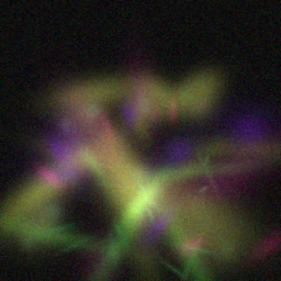
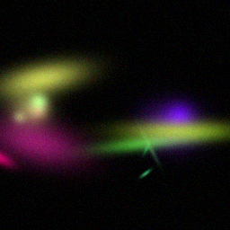
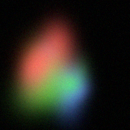
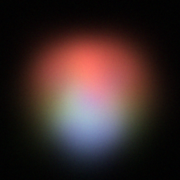
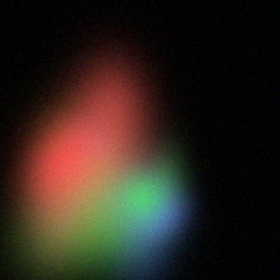
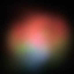
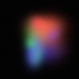
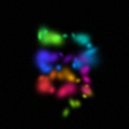
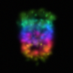
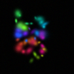
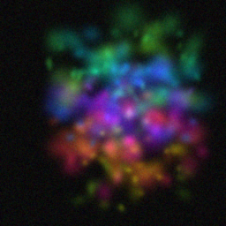
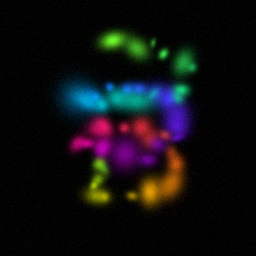
Reconstruction Gallery — 4 Scenes × 3 Scenarios

Method: CPU_baseline | Mismatch: nominal (nominal=True, perturbed=False)

I Ideal II Mismatch (uncorrected) III Oracle correction

I — Ideal

Ground Truth

Measurement

Reconstruction

13.554075184041242 dB SSIM 0.7184238727633953

II — Mismatch

Ground Truth

Measurement

Reconstruction

13.39628622336437 dB SSIM 0.6941699782424309

III — Oracle

Ground Truth

Measurement (perturbed)

Reconstruction

11.264981514394965 dB SSIM 0.4810473177289441

I — Ideal

Ground Truth

Measurement

Reconstruction

11.406260010627813 dB SSIM 0.19612763121173293

II — Mismatch

Ground Truth

Measurement

Reconstruction

13.084516541904206 dB SSIM 0.11534430736937398

III — Oracle

Ground Truth

Measurement (perturbed)

Reconstruction

13.992298722668512 dB SSIM 0.3354100240330721

I — Ideal

Ground Truth

Measurement

Reconstruction

19.571561352139778 dB SSIM 0.623308435153531

II — Mismatch

Ground Truth

Measurement

Reconstruction

17.910878938411106 dB SSIM 0.5565384225062122

III — Oracle

Ground Truth

Measurement (perturbed)

Reconstruction

16.22944882101815 dB SSIM 0.41338047490987834

I — Ideal

Ground Truth

Measurement

Reconstruction

20.36229989072771 dB SSIM 0.4161772858606524

II — Mismatch

Ground Truth

Measurement

Reconstruction

17.30560964431787 dB SSIM 0.0916963151505076

III — Oracle

Ground Truth

Measurement (perturbed)

Reconstruction

17.937224860688367 dB SSIM 0.4288107354552466

Mean PSNR Across All Scenes

16.223549109384138 dB

I — Ideal

15.424322836999387 dB

II — Mismatch

14.855988479692497 dB

III — Oracle

Degradation: -0.8 dB Recovery: +-0.6 dB

Per-scene PSNR breakdown (4 scenes)

Scene	I (PSNR)	I (SSIM)	II (PSNR)	II (SSIM)	III (PSNR)	III (SSIM)
scene_00	13.554075184041242	0.7184238727633953	13.39628622336437	0.6941699782424309	11.264981514394965	0.4810473177289441
scene_01	11.406260010627813	0.19612763121173293	13.084516541904206	0.11534430736937398	13.992298722668512	0.3354100240330721
scene_02	19.571561352139778	0.623308435153531	17.910878938411106	0.5565384225062122	16.22944882101815	0.41338047490987834
scene_03	20.36229989072771	0.4161772858606524	17.30560964431787	0.0916963151505076	17.937224860688367	0.4288107354552466
Mean	16.223549109384138	0.4885093062473279	15.424322836999387	0.36443725581713116	14.855988479692497	0.4146621380317853

Experimental Setup

Training Views: 24-300 (scene-dependent)

Image Resolution: ~1600x1200

Initialization: SfM point cloud (COLMAP)

Rendering Fps: 30

Scene Type: unbounded indoor / outdoor

Training Iterations: 30000

Evaluation: PSNR / SSIM / LPIPS

Dataset: Mip-NeRF360, Tanks & Temples, Deep Blending

Key References

Kerbl et al., '3D Gaussian Splatting for Real-Time Radiance Field Rendering', SIGGRAPH 2023

Canonical Datasets

Mip-NeRF 360 (9 scenes)
Tanks & Temples (Knapitsch et al.)
Deep Blending (Hedman et al.)

Spec DAG — Forward Model Pipeline

Π(splat) → Σ(alpha) → D(g, η₁)

Π Gaussian Splatting (splat)

Σ Alpha Compositing (alpha)

D Camera (g, η₁)

Mismatch Parameters

Symbol	Parameter	Description	Perturbed
ΔT	camera_pose	Camera pose error (mm / deg)	1.0
Δf	focal_length	Focal length error (pixels)	5.0
ΔP	point_cloud_init	Initial point cloud noise (mm)	2.0

Credits System

40%

Platform Profit Pool

Revenue allocated to benchmark rewards

30%

Winner Share

Top algorithm receives from pool

$100

Min Withdrawal

Minimum payout threshold

Spec Primitives Reference (11 primitives)

P Propagation

Free-space or medium propagation kernel (Fresnel, Rayleigh-Sommerfeld).

M Mask / Modulation

Spatial or spatio-temporal amplitude modulation (coded aperture, SLM pattern).

Π Projection

Geometric projection operator (Radon transform, fan-beam, cone-beam).

F Fourier Sampling

Sampling in the Fourier / k-space domain (MRI, ptychography).

C Convolution

Shift-invariant convolution with a point-spread function (PSF).

Σ Summation / Integration

Summation along a physical dimension (spectral, temporal, angular).

D Detector

Sensor readout with gain g and noise model η (Gaussian, Poisson, mixed).

S Structured Illumination

Patterned illumination (block, Hadamard, random) applied to the scene.

W Wavelength Dispersion

Spectral dispersion element (prism, grating) with shift α and aperture a.

R Rotation / Motion

Sample or gantry rotation (CT, electron tomography).

Λ Wavelength Selection

Spectral filter or monochromator selecting a wavelength band.