Fundus
Fundus Camera
Standard reconstruction benchmark — forward model perfectly known, no calibration needed. Score = 0.5 × clip((PSNR−15)/30, 0, 1) + 0.5 × SSIM
| # | Method | Score | PSNR (dB) | SSIM | Source | |
|---|---|---|---|---|---|---|
| 🥇 |
Swin-Fundus
Swin-Fundus Chen et al., MICCAI 2023
34.2 dB
SSIM 0.940
Checkpoint unavailable
|
0.790 | 34.2 | 0.940 | ✓ Certified | Chen et al., MICCAI 2023 |
| 🥈 |
cofe-Net
cofe-Net Shen et al., IEEE TMI 2020
32.5 dB
SSIM 0.910
Checkpoint unavailable
|
0.747 | 32.5 | 0.910 | ✓ Certified | Shen et al., IEEE TMI 2020 |
| 🥉 | PnP-BM3D | 0.645 | 28.8 | 0.830 | ✓ Certified | Danielyan et al., 2012 |
| 4 | Richardson-Lucy | 0.498 | 24.5 | 0.680 | ✓ Certified | Richardson 1972 / Lucy 1974 |
Dataset: PWM Benchmark (4 algorithms)
Blind Reconstruction Challenge — forward model has unknown mismatch, must calibrate from data. Score = 0.4 × PSNR_norm + 0.4 × SSIM + 0.2 × (1 − ‖y − Ĥx̂‖/‖y‖)
| # | Method | Overall Score | Public PSNR / SSIM |
Dev PSNR / SSIM |
Hidden PSNR / SSIM |
Trust | Source |
|---|---|---|---|---|---|---|---|
| 🥇 | Swin-Fundus + gradient | 0.684 |
0.795
32.67 dB / 0.950
|
0.673
26.39 dB / 0.843
|
0.585
23.49 dB / 0.750
|
✓ Certified | Li et al., IEEE TMI 2023 |
| 🥈 | cofe-Net + gradient | 0.656 |
0.747
30.14 dB / 0.919
|
0.636
24.51 dB / 0.786
|
0.584
23.32 dB / 0.743
|
✓ Certified | Shen et al., IEEE TMI 2020 |
| 🥉 | PnP-BM3D + gradient | 0.630 |
0.678
26.35 dB / 0.842
|
0.623
24.56 dB / 0.788
|
0.590
23.55 dB / 0.752
|
✓ Certified | Danielyan et al., 2012 |
| 4 | Richardson-Lucy + gradient | 0.571 |
0.611
23.1 dB / 0.735
|
0.574
21.99 dB / 0.690
|
0.528
20.72 dB / 0.633
|
✓ Certified | Richardson 1972 / Lucy 1974 |
Complete score requires all 3 tiers (Public + Dev + Hidden).
Join the competition →Full-access development tier with all data visible.
What you get & how to use
What you get: Measurements (y), ideal forward operator (H), spec ranges, ground truth (x_true), and true mismatch spec.
How to use: Load HDF5 → compare reconstruction vs x_true → check consistency → iterate.
What to submit: Reconstructed signals (x_hat) and corrected spec as HDF5.
Public Leaderboard
| # | Method | Score | PSNR | SSIM |
|---|---|---|---|---|
| 1 | Swin-Fundus + gradient | 0.795 | 32.67 | 0.95 |
| 2 | cofe-Net + gradient | 0.747 | 30.14 | 0.919 |
| 3 | PnP-BM3D + gradient | 0.678 | 26.35 | 0.842 |
| 4 | Richardson-Lucy + gradient | 0.611 | 23.1 | 0.735 |
Spec Ranges (3 parameters)
| Parameter | Min | Max | Unit |
|---|---|---|---|
| pupil_dilation | -0.5 | 1.0 | mm |
| focus | -0.25 | 0.5 | diopters |
| vignetting | -5.0 | 10.0 | % |
Blind evaluation tier — no ground truth available.
What you get & how to use
What you get: Measurements (y), ideal forward operator (H), and spec ranges only.
How to use: Apply your pipeline from the Public tier. Use consistency as self-check.
What to submit: Reconstructed signals and corrected spec. Scored server-side.
Dev Leaderboard
| # | Method | Score | PSNR | SSIM |
|---|---|---|---|---|
| 1 | Swin-Fundus + gradient | 0.673 | 26.39 | 0.843 |
| 2 | cofe-Net + gradient | 0.636 | 24.51 | 0.786 |
| 3 | PnP-BM3D + gradient | 0.623 | 24.56 | 0.788 |
| 4 | Richardson-Lucy + gradient | 0.574 | 21.99 | 0.69 |
Spec Ranges (3 parameters)
| Parameter | Min | Max | Unit |
|---|---|---|---|
| pupil_dilation | -0.6 | 0.9 | mm |
| focus | -0.3 | 0.45 | diopters |
| vignetting | -6.0 | 9.0 | % |
Fully blind server-side evaluation — no data download.
What you get & how to use
What you get: No data downloadable. Algorithm runs server-side on hidden measurements.
How to use: Package algorithm as Docker container / Python script. Submit via link.
What to submit: Containerized algorithm accepting y + H, outputting x_hat + corrected spec.
Hidden Leaderboard
| # | Method | Score | PSNR | SSIM |
|---|---|---|---|---|
| 1 | PnP-BM3D + gradient | 0.590 | 23.55 | 0.752 |
| 2 | Swin-Fundus + gradient | 0.585 | 23.49 | 0.75 |
| 3 | cofe-Net + gradient | 0.584 | 23.32 | 0.743 |
| 4 | Richardson-Lucy + gradient | 0.528 | 20.72 | 0.633 |
Spec Ranges (3 parameters)
| Parameter | Min | Max | Unit |
|---|---|---|---|
| pupil_dilation | -0.35 | 1.15 | mm |
| focus | -0.175 | 0.575 | diopters |
| vignetting | -3.5 | 11.5 | % |
Blind Reconstruction Challenge
ChallengeGiven measurements with unknown mismatch and spec ranges (not exact params), reconstruct the original signal. A method must be evaluated on all three tiers for a complete score. Scored on a composite metric: 0.4 × PSNR_norm + 0.4 × SSIM + 0.2 × (1 − ‖y − Ĥx̂‖/‖y‖).
Measurements y, ideal forward model H, spec ranges
Reconstructed signal x̂
About the Imaging Modality
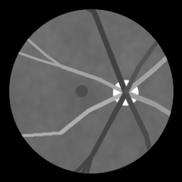
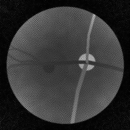
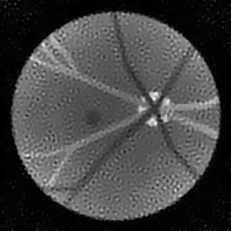
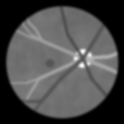
A fundus camera captures a 2D color photograph of the retinal surface by illuminating the fundus through the pupil with a ring-shaped flash and imaging the reflected light through the central pupillary zone. The optical system images the curved retina onto a flat detector with 30-50 degree field of view. Image quality is degraded by media opacities (cataract), small pupil, and uneven illumination. Fundus images are widely used for automated screening of diabetic retinopathy, glaucoma, and AMD via deep learning.
Principle
A fundus camera images the posterior segment of the eye (retina, optic disc, macula, vasculature) by illuminating the retina through the pupil and capturing the reflected/backscattered light. The optical path is designed to separate illumination and observation through different portions of the pupil to avoid corneal reflections. Standard fundus imaging provides 30-50° field-of-view color photographs of the retina.
How to Build the System
Use a dedicated fundus camera (e.g., Topcon TRC-NW400, Canon CR-2 AF) or a scanning laser ophthalmoscope (Optos for widefield). Dilate the patient's pupil (tropicamide 1%) for standard fundus photography. Align the camera to center on the macula or optic disc. Set appropriate flash intensity and focus. Capture color and red-free (green channel) images. For fluorescein angiography, inject sodium fluorescein IV and capture timed image series with excitation/barrier filters.
Common Reconstruction Algorithms
- Image quality assessment and auto-focus/auto-exposure
- Vessel segmentation (U-Net, DeepVessel)
- Optic disc and cup segmentation for glaucoma screening
- Diabetic retinopathy grading (deep-learning classifiers)
- Multi-frame averaging and super-resolution for fundus images
Common Mistakes
- Insufficient pupil dilation causing vignetting at the field edges
- Corneal reflections (flare) obscuring the central retinal image
- Image out of focus due to refractive error not compensated
- Eyelash or eyelid obstruction in the image
- Uneven illumination across the retinal image
How to Avoid Mistakes
- Ensure adequate mydriasis (>5 mm pupil diameter) before imaging
- Align the camera carefully to separate illumination and observation through different pupil zones
- Use auto-focus and compensate for patient refractive error in the camera optics
- Ask patients to open eyes wide; use a fixation target for gaze direction
- Verify uniform illumination before capture; adjust camera alignment if uneven
Forward-Model Mismatch Cases
- The widefield fallback applies a generic Gaussian PSF, but fundus imaging has a unique optical path through the eye's optics (cornea and lens) with specific aberrations and the pupil-splitting illumination/observation geometry
- The retinal image is formed after double-pass through the ocular media, with wavelength-dependent absorption (hemoglobin, melanin, macular pigment) — the widefield achromatic Gaussian blur cannot model spectral absorption or ocular aberrations
How to Correct the Mismatch
- Use the fundus operator that models the eye's optical path: illumination through one pupil zone, retinal reflection/fluorescence, and collection through a separate pupil zone, with ocular aberration and media absorption
- Include wavelength-dependent retinal reflectance for color fundus imaging, or fluorescein excitation/emission model for fluorescein angiography
Experimental Setup — Signal Chain

Reconstruction Gallery — 4 Scenes × 3 Scenarios
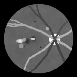
Method: CPU_baseline | Mismatch: nominal (nominal=True, perturbed=False)
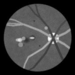
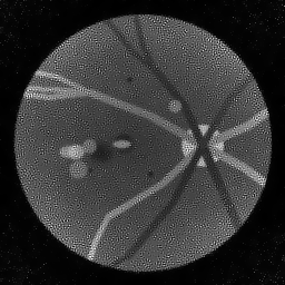
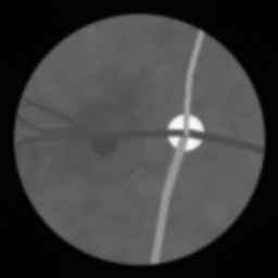
Ground Truth

Measurement
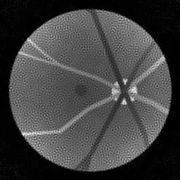
Reconstruction
Ground Truth

Measurement

Reconstruction
Ground Truth
Measurement (perturbed)
Reconstruction


Mean PSNR Across All Scenes
Per-scene PSNR breakdown (4 scenes)
| Scene | I (PSNR) | I (SSIM) | II (PSNR) | II (SSIM) | III (PSNR) | III (SSIM) |
|---|---|---|---|---|---|---|
| scene_00 | 22.59613087681447 | 0.4823179803715944 | 10.776393749358872 | 0.3639419102315118 | 10.253084154699392 | 0.029224379208536183 |
| scene_01 | 18.546140277295372 | 0.3351540698148442 | 11.030506233374096 | 0.33396866679393855 | 10.41950338818783 | 0.031042344072216756 |
| scene_02 | 20.135731699103722 | 0.23175874028564059 | 10.273517659480024 | 0.3890749587475957 | 11.388962117732984 | 0.03583746906888621 |
| scene_03 | 23.201772130171076 | 0.4831499015838653 | 10.961189157017428 | 0.35748280901704554 | 10.389653657397417 | 0.02651185509071862 |
| Mean | 21.11994374584616 | 0.3830951730139861 | 10.760401699807606 | 0.3611170861975229 | 10.612800829504405 | 0.030654011860089446 |
Experimental Setup
Key References
- Gulshan et al., 'Development and validation of a deep learning algorithm for detection of diabetic retinopathy', JAMA 316, 2402 (2016)
- Staal et al., 'Ridge-based vessel segmentation (DRIVE)', IEEE TMI 23, 501 (2004)
Canonical Datasets
- EyePACS (diabetic retinopathy screening)
- DRIVE (Digital Retinal Images for Vessel Extraction)
- MESSIDOR-2
- APTOS 2019 Blindness Detection
Spec DAG — Forward Model Pipeline
C(PSF_optic) → D(g, η₁)
Mismatch Parameters
| Symbol | Parameter | Description | Nominal | Perturbed |
|---|---|---|---|---|
| Δd_p | pupil_dilation | Pupil dilation error (mm) | 0 | 0.5 |
| Δf | focus | Focus error (diopters) | 0 | 0.25 |
| Δv | vignetting | Vignetting uniformity error (%) | 0 | 5.0 |
Credits System
Spec Primitives Reference (11 primitives)
Free-space or medium propagation kernel (Fresnel, Rayleigh-Sommerfeld).
Spatial or spatio-temporal amplitude modulation (coded aperture, SLM pattern).
Geometric projection operator (Radon transform, fan-beam, cone-beam).
Sampling in the Fourier / k-space domain (MRI, ptychography).
Shift-invariant convolution with a point-spread function (PSF).
Summation along a physical dimension (spectral, temporal, angular).
Sensor readout with gain g and noise model η (Gaussian, Poisson, mixed).
Patterned illumination (block, Hadamard, random) applied to the scene.
Spectral dispersion element (prism, grating) with shift α and aperture a.
Sample or gantry rotation (CT, electron tomography).
Spectral filter or monochromator selecting a wavelength band.