FPM
Fourier Ptychographic Microscopy
Standard reconstruction benchmark — forward model perfectly known, no calibration needed. Score = 0.5 × clip((PSNR−15)/30, 0, 1) + 0.5 × SSIM
| # | Method | Score | PSNR (dB) | SSIM | Source | |
|---|---|---|---|---|---|---|
| 🥇 |
PtychoDV
PtychoDV Shamshad et al., IEEE TCI 2019
33.8 dB
SSIM 0.935
Checkpoint unavailable
|
0.781 | 33.8 | 0.935 | ✓ Certified | Shamshad et al., IEEE TCI 2019 |
| 🥈 |
Fourier PtychoNet
Fourier PtychoNet Jiang et al., BOE 2018
32.3 dB
SSIM 0.910
Checkpoint unavailable
|
0.743 | 32.3 | 0.910 | ✓ Certified | Jiang et al., BOE 2018 |
| 🥉 | Gradient Descent FPM | 0.645 | 28.5 | 0.840 | ✓ Certified | Tian & Waller, Optica 2015 |
| 4 | Alternating Projections | 0.527 | 25.0 | 0.720 | ✓ Certified | Zheng et al., Nat. Photonics 2013 |
Dataset: PWM Benchmark (4 algorithms)
Blind Reconstruction Challenge — forward model has unknown mismatch, must calibrate from data. Score = 0.4 × PSNR_norm + 0.4 × SSIM + 0.2 × (1 − ‖y − Ĥx̂‖/‖y‖)
| # | Method | Overall Score | Public PSNR / SSIM |
Dev PSNR / SSIM |
Hidden PSNR / SSIM |
Trust | Source |
|---|---|---|---|---|---|---|---|
| 🥇 | PtychoDV + gradient | 0.679 |
0.766
31.38 dB / 0.936
|
0.653
26.11 dB / 0.835
|
0.618
24.68 dB / 0.792
|
✓ Certified | Shamshad et al., IEEE TCI 2019 |
| 🥈 | Gradient Descent FPM + gradient | 0.656 |
0.666
25.51 dB / 0.818
|
0.660
26.31 dB / 0.841
|
0.643
25.08 dB / 0.805
|
✓ Certified | Tian & Waller, Optica 2015 |
| 🥉 | Fourier PtychoNet + gradient | 0.592 |
0.741
29.65 dB / 0.911
|
0.580
22.74 dB / 0.721
|
0.455
18.84 dB / 0.542
|
✓ Certified | Jiang et al., BOE 2018 |
| 4 |
Alternating Projections + gradient
Alternating Projections + gradient Zheng et al., Nat. Photonics 2013 Score 0.566
Correct & Reconstruct →
|
0.566 |
0.620
23.29 dB / 0.742
|
0.568
22.16 dB / 0.697
|
0.511
19.91 dB / 0.594
|
✓ Certified | Zheng et al., Nat. Photonics 2013 |
Complete score requires all 3 tiers (Public + Dev + Hidden).
Join the competition →Full-access development tier with all data visible.
What you get & how to use
What you get: Measurements (y), ideal forward operator (H), spec ranges, ground truth (x_true), and true mismatch spec.
How to use: Load HDF5 → compare reconstruction vs x_true → check consistency → iterate.
What to submit: Reconstructed signals (x_hat) and corrected spec as HDF5.
Public Leaderboard
| # | Method | Score | PSNR | SSIM |
|---|---|---|---|---|
| 1 | PtychoDV + gradient | 0.766 | 31.38 | 0.936 |
| 2 | Fourier PtychoNet + gradient | 0.741 | 29.65 | 0.911 |
| 3 | Gradient Descent FPM + gradient | 0.666 | 25.51 | 0.818 |
| 4 | Alternating Projections + gradient | 0.620 | 23.29 | 0.742 |
Spec Ranges (3 parameters)
| Parameter | Min | Max | Unit |
|---|---|---|---|
| led_position | -0.1 | 0.2 | mm |
| na_error | 0.095 | 0.11 | |
| defocus | -2.0 | 4.0 | μm |
Blind evaluation tier — no ground truth available.
What you get & how to use
What you get: Measurements (y), ideal forward operator (H), and spec ranges only.
How to use: Apply your pipeline from the Public tier. Use consistency as self-check.
What to submit: Reconstructed signals and corrected spec. Scored server-side.
Dev Leaderboard
| # | Method | Score | PSNR | SSIM |
|---|---|---|---|---|
| 1 | Gradient Descent FPM + gradient | 0.660 | 26.31 | 0.841 |
| 2 | PtychoDV + gradient | 0.653 | 26.11 | 0.835 |
| 3 | Fourier PtychoNet + gradient | 0.580 | 22.74 | 0.721 |
| 4 | Alternating Projections + gradient | 0.568 | 22.16 | 0.697 |
Spec Ranges (3 parameters)
| Parameter | Min | Max | Unit |
|---|---|---|---|
| led_position | -0.12 | 0.18 | mm |
| na_error | 0.094 | 0.109 | |
| defocus | -2.4 | 3.6 | μm |
Fully blind server-side evaluation — no data download.
What you get & how to use
What you get: No data downloadable. Algorithm runs server-side on hidden measurements.
How to use: Package algorithm as Docker container / Python script. Submit via link.
What to submit: Containerized algorithm accepting y + H, outputting x_hat + corrected spec.
Hidden Leaderboard
| # | Method | Score | PSNR | SSIM |
|---|---|---|---|---|
| 1 | Gradient Descent FPM + gradient | 0.643 | 25.08 | 0.805 |
| 2 | PtychoDV + gradient | 0.618 | 24.68 | 0.792 |
| 3 | Alternating Projections + gradient | 0.511 | 19.91 | 0.594 |
| 4 | Fourier PtychoNet + gradient | 0.455 | 18.84 | 0.542 |
Spec Ranges (3 parameters)
| Parameter | Min | Max | Unit |
|---|---|---|---|
| led_position | -0.07 | 0.23 | mm |
| na_error | 0.0965 | 0.1115 | |
| defocus | -1.4 | 4.6 | μm |
Blind Reconstruction Challenge
ChallengeGiven measurements with unknown mismatch and spec ranges (not exact params), reconstruct the original signal. A method must be evaluated on all three tiers for a complete score. Scored on a composite metric: 0.4 × PSNR_norm + 0.4 × SSIM + 0.2 × (1 − ‖y − Ĥx̂‖/‖y‖).
Measurements y, ideal forward model H, spec ranges
Reconstructed signal x̂
About the Imaging Modality
Fourier ptychographic microscopy (FPM) achieves a high space-bandwidth product by illuminating the sample from multiple angles using an LED array, capturing a set of low-resolution images, and computationally stitching them in Fourier space to synthesize a high-NA image with both amplitude and phase. Each LED angle shifts the sample's spatial frequency spectrum in Fourier space, and overlapping spectral regions provide redundancy for phase retrieval. The synthetic NA equals the objective NA plus the illumination NA. Reconstruction uses iterative phase retrieval algorithms (sequential or gradient-based).
Principle
Fourier Ptychographic Microscopy synthetically increases the NA of a low-magnification objective by illuminating the sample from multiple angles (LED array) and computationally stitching together the resulting images in Fourier space. Each LED angle shifts the sample spectrum so different spatial-frequency bands enter the objective pupil, allowing recovery of both amplitude and phase at high resolution over a large field of view.
How to Build the System
Replace the microscope condenser with a programmable LED matrix (e.g., 32×32 RGB LED array, ~4 mm pitch, placed ~80 mm above the sample). Use a low-magnification objective (4-10×, 0.1-0.3 NA) for large FOV. Acquire one image per LED (typically 100-300 images for the full matrix). Precise knowledge of LED positions is required for Fourier-space stitching.
Common Reconstruction Algorithms
- Alternating projection (Gerchberg-Saxton style in Fourier space)
- Embedded pupil function recovery (joint sample + aberration estimation)
- Wirtinger gradient descent with total-variation regularization
- Neural network-accelerated FPM (learned initialization + refinement)
- Multiplexed FPM (multiple LEDs simultaneously for faster acquisition)
Common Mistakes
- Inaccurate LED position calibration causing ghosting and resolution loss
- Insufficient overlap between Fourier-space patches (need ≥60 % overlap)
- Ignoring pupil aberrations of the low-NA objective
- LED intensity non-uniformity not corrected across the array
- Vibration or sample drift between sequential LED acquisitions
How to Avoid Mistakes
- Calibrate LED positions using a self-calibration algorithm or known test target
- Ensure adequate angular spacing to maintain >60% Fourier overlap between adjacent LEDs
- Use embedded pupil recovery to jointly estimate and correct aberrations
- Normalize LED intensities with a blank-sample calibration acquisition
- Stabilize the setup mechanically; use fast cameras to minimize inter-frame drift
Forward-Model Mismatch Cases
- The widefield fallback produces a single (64,64) image, but FPM acquires 25+ images from different LED illumination angles — output shape (25,16,16) captures distinct spatial-frequency bands for each angle
- FPM is fundamentally nonlinear (intensity = |F^-1{P * F{O * exp(i*k_led*r)}}|^2) — the widefield linear blur cannot model the coherent pupil filtering and phase recovery that enables synthetic aperture
How to Correct the Mismatch
- Use the FPM operator that generates one low-resolution intensity image per LED angle, each capturing a different region of the sample's Fourier spectrum shifted by the illumination wavevector
- Reconstruct using alternating projection (Gerchberg-Saxton in Fourier space) or embedded pupil recovery, which require the correct coherent forward model with known LED positions
Experimental Setup — Signal Chain

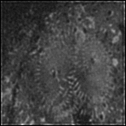
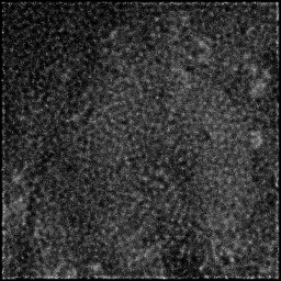
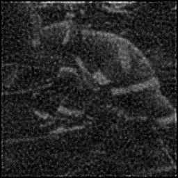
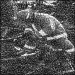
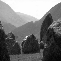
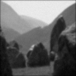
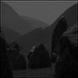
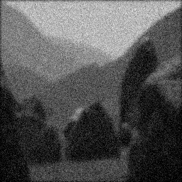
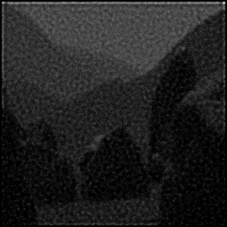
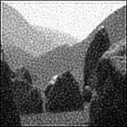
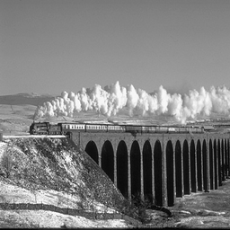
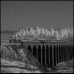
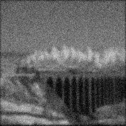
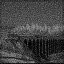
Reconstruction Gallery — 4 Scenes × 3 Scenarios
Method: CPU_baseline | Mismatch: nominal (nominal=True, perturbed=False)

Ground Truth
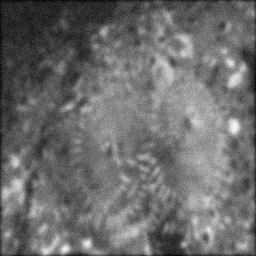
Measurement
Reconstruction
Ground Truth

Measurement
Reconstruction
Ground Truth
Measurement (perturbed)
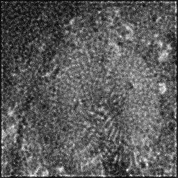
Reconstruction


Mean PSNR Across All Scenes
Per-scene PSNR breakdown (4 scenes)
| Scene | I (PSNR) | I (SSIM) | II (PSNR) | II (SSIM) | III (PSNR) | III (SSIM) |
|---|---|---|---|---|---|---|
| scene_00 | 17.022206064497794 | 0.38380508849556166 | 14.005042899600344 | 0.20435053699637695 | 18.90867036945368 | 0.43244231803409233 |
| scene_01 | 14.231375949985203 | 0.29689664293183293 | 12.51886569801027 | 0.1837236295719222 | 18.36836409325208 | 0.48764883686484906 |
| scene_02 | 8.520061941863302 | 0.3871062840596513 | 7.895669461330657 | 0.1975567523194643 | 19.167062537286945 | 0.2761352350679213 |
| scene_03 | 13.297073801541249 | 0.5284335563352818 | 11.313290229125483 | 0.22807457115490956 | 18.62930373252439 | 0.38602598080736633 |
| Mean | 13.267679439471888 | 0.39906039295558193 | 11.433217072016689 | 0.20342637251066828 | 18.76835018312927 | 0.39556309269355727 |
Experimental Setup
Key References
- Zheng et al., 'Wide-field, high-resolution Fourier ptychographic microscopy', Nature Photonics 7, 739-745 (2013)
- Tian & Waller, 'Quantitative differential phase contrast imaging in an LED array microscope', Optics Express 23, 11394-11403 (2015)
Canonical Datasets
- Zheng lab FPM datasets (UCONN)
- Waller lab FPM benchmark data (Berkeley)
Spec DAG — Forward Model Pipeline
S(LED array) → C(PSF_NA) → Σ_θ → D(g, η₁)
Mismatch Parameters
| Symbol | Parameter | Description | Nominal | Perturbed |
|---|---|---|---|---|
| Δr_LED | led_position | LED position error (mm) | 0 | 0.1 |
| ΔNA | na_error | Numerical aperture error | 0.1 | 0.105 |
| Δz | defocus | Defocus error (μm) | 0 | 2.0 |
Credits System
Spec Primitives Reference (11 primitives)
Free-space or medium propagation kernel (Fresnel, Rayleigh-Sommerfeld).
Spatial or spatio-temporal amplitude modulation (coded aperture, SLM pattern).
Geometric projection operator (Radon transform, fan-beam, cone-beam).
Sampling in the Fourier / k-space domain (MRI, ptychography).
Shift-invariant convolution with a point-spread function (PSF).
Summation along a physical dimension (spectral, temporal, angular).
Sensor readout with gain g and noise model η (Gaussian, Poisson, mixed).
Patterned illumination (block, Hadamard, random) applied to the scene.
Spectral dispersion element (prism, grating) with shift α and aperture a.
Sample or gantry rotation (CT, electron tomography).
Spectral filter or monochromator selecting a wavelength band.